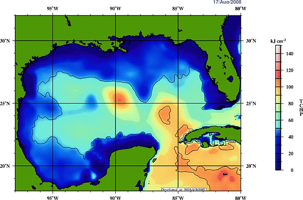
Tropical Cyclone Heat Potential
Methodology
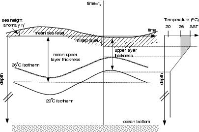
Sea surface temperature (SST) provides a measure of the surface ocean conditions, however no information about the subsurface ocean thermal structure (approximately the upper 50 m of the ocean) can be derived from SST alone. For instance, it is known that the oceanic skin temperature erodes when the sea surface is affected by strong winds, creating a well-mixed layer that can reach depths of several tens of meters. Moreover, warm ocean features, mainly anticyclonic rings and eddies, are characterized by a deepening of the isotherms towards their centers with a markedly different temperature and salinity structure than the surrounding waters. Several studies have shown that observations of sea surface height (SSH) are strongly correlated with the thermal structure of the upper ocean (e.g. Goni et al. 1996; Gilson et al. 1998; Mayer et al. 2001; Willis et al. 2004). Based in this virtually ubiquitous relationship, we developed a methodology to estimate fields of isotherm depth from the SHA fields derived from satellite observations.
The tropical cyclone heat potential (hereafter TCHP), is defined as a measure of the integrated vertical temperature from the sea surface to the depth of the 26℃ isotherm. This parameter is computed globally from the altimeter-derived vertical temperature profiles estimates in the upper ocean (Shay et al., 2000). Different methods have been developed to calculate this vertical thermal structure of the upper ocean. Up to three different procedures have been developed at NOAA/AOML for this purpose. In chronological order, the first TCHP fields were obtained using a reduced-gravity model (Version 1.0). In May 2005, a second algorithm based on linear regression analysis (Version 2.0) was implemented and all the fields available through this website were updated accordingly. Finally, in October 2008, a third approach was put into service, in order to provide better agreement with observations and remove outliers mainly affecting the Gulf of America and Central Pacific regions (Version 2.1).
| Methodology Version | Time Period |
|---|---|
| 1.0 | Before Jan/01/2005 |
| 2.0 | Jan/01/2005-Oct/14/2008 |
| 2.1 | Oct/15/2008-Present |
The sea height anomaly (SHA) represents the deviation of the sea height with respect to its mean. Sea height anomaly fields from the altimeter constellation, are used in this study. For analysis and corrections of altimeter data, please refer to: Cheney et al, TOPEX/POSEIDON: The 2-cm Solution, J. Geophys. Res., 99, 24555-24564, 1994.
In this page, we present four daily maps: sea height anomalies, sea surface temperature, altimeter-estimate of the depth of the 26℃ isotherm and TCHP. These maps can be used to identify warm anticyclonic features, usually characterized by sea height anomalies and a depth of the 26℃ isotherm larger than their surrounding waters; and to monitor regions of very high (usually larger than 90 kJ cm-2) TCHP. These regions have been associated with the sudden intensification of tropical cyclones.
The role of the ocean in tropical cyclone (TC) formation has been largely recognized and accepted. A strong link has been identified between high TCHP values and intensification of TCs (e.g. Shay et al. 2000, Maineli et al. 2008). Hydrographic observations cannot provide TCHP fields needed to monitor this key parameter on a daily to weekly basis with wide coverage over regions of TC activity. Daily global fields of TCHP are obtained integrating the thermal structure derived from the satellite observations down to the 26℃ isotherm. In the Gulf of America, high values of TCHP are typically associated with the Loop Current and Anticyclonic Rings (see figure below).
 |
Version 1.0
The close relationship that exists between the dynamic height and the mass field of the ocean allows these two parameters to be used within a two-layer reduced gravity ocean model to monitor the upper layer thickness (Goni et al., 1996), which is defined in this study to go from the sea surface to the depth of the 20℃ isotherm. This isotherm is chosen because it lies within the center of the main thermocline and is often used as an indicator of the upper layer flow in the western tropical Atlantic and Gulf of America waters. Although there are other factors controlling the sea height anomaly, it is assumed here that most of its variability is due to changes in the depth of the main thermocline and of barotropic origin. In this method the temperature profiles are estimated using three points: (a) the sea surface temperature obtained from the Tropical Rainfall Measuring Mission's (TRMM) Microwave Imager (TMI) fields, (b) the altimeter-estimates of the 20℃ isotherm within a two-layer reduced gravity scheme (Goni et al, 1996), (c) the depth of the 26℃ isotherm from a climatological relationship between the depths of the 20℃ and 26℃ isotherm.
 |
Maps created using this algorithm are no longer available on this website.
Version 2.0
All the maps were reprocessed using a new algorithm based on the linear regression between the depth of the isotherms from 26℃ to 28℃, as obtained from temperature profiles, and the dynamic topography estimated from altimetry by AVISO. The mean dynamic field is the Rio05 Combined Mean Dynamic Topography . The slope and intercept factors for each isotherm were calculated for each cell of 2x2 degree using the values falling within a radius of 2.5° degrees from each cell center. The TCHP values were then obtained from integrating the resulting temperature profile from the surface to the depth of the 26℃ isotherm. The SST field was provided on a daily basis by Remote Sensing Systems and was obtained from TMI MW measuremens for a latitude band between 40N and 40S.
Version 2.1
This methodology estimates the fields of isotherm depth from the SHA retrievals obtained from satellite observations. The algorithm steps are the following:
- - In-situ temperature profiles obtained mostly from eXpendable BathyThermograph and profiling-float observations from 1992 to 2006 are grouped in 3° x 3° bins with a 1° x 1° resolution.
- - The depth of the 26℃ to 28℃ isotherms is estimated from each profile.
- - The weekly SHA gridded fields derived by AVISO are interpolated into the location and time of the temperature profiles.
- - In each 1° x 1° bin the depth of each isotherm is linearly regressed onto the corresponding SHA value.
- - Only regression parameters that are statistically significant within a 1-sigma level are considered. Any small gaps in the resulting fields of regression parameters are interpolated.
- - In each 1° x 1° bin a synthetic temperature profile is derived from the regression parameters and the daily real-time SHA fields distributed by AVISO. These synthetic profiles are completed with global TMI-AMSR-E SST fields for the z = 0 temperature.
- - The TCHP field, the anomalous heat storage associated with temperatures larger than 26℃, is computed from each synthetic temperature profile.