3.2 Models of the ventilated thermocline

Model description: Models of the ventilated thermocline are based on the Sverdrup dynamics. In contrast to the simple Sverdrup model, however, they resolve the circulation in the vertical. One way to implement a vertical discretization is the introduction of several layers between the surface mixed layer and a stagnant layer (Fig.   10  , Luyten et al., 1983; Luyten and Stommel, 1986; Pedlosky and Robbins, 1991). The layers are driven by Ekman pumping in those regions where they intersect the upper boundary. Negative (downward) vertical Ekman velocity, which is typical for the subtropical regions, causes a ventilation of the uppermost layer. Hereby, this layer gains a certain amount of potential vorticity which is conserved once the layer is subducted under another layer. The potential vorticity conservation causes an anticyclonic circulation in the subducted layer, similar to that in the uppermost layer. With increasing depth the center of the anticyclonic gyre shifts towards the nearest pole. The velocities in the individual layers are in geostrophic balance.

One important assumption of the models is that only those layers which are the uppermost layer in a region with downward Ekman pumping are governed by the wind-driven gyre circulation. We showed in section 2 that a subduction of SAMW into the AAIW layer is possible. This conclusion is supported by the thickness of the Ekman layer ($D_E = \pi \sqrt{(2 \cdot A_z / \vert f\vert)}$, with A_z = vertical turbulent viscosity and f = Coriolis parameter). In the PFZ (between 45^oS and 50^oS) the Ekman depth is about 100 mfor a vertical turbulent viscosity of 0.05 m²s^-1 (published values range from 10^-4 to 10^-1  m²s^-1, Wang et al., 1996). This estimate corresponds well with the mixed layer depth in this region. Also the vertical Ekman velocity in the PFZ is frequently directed downward. We therefore conclude that the hydrographic observations and the wind field patterns support the hypothesis of subduction in the PFZ.

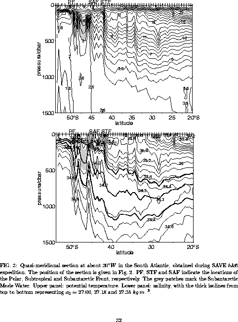
The results obtained by Ribbe and Tomczak (1997) with the Fine Resolution Antarctic Model (FRAM) provide further evidence that a wind-induced ventilation of AAIW is possible in the PFZ of the South Atlantic. In FRAM 65% of the water in 532 m at 44^oS originates in the PFZ, whereas only 35% originate in the near-surface layer of the Antarctic Zone. The depth of 532 m is approximately the observed depth of the AAIW core layer near 44^oS (Fig.  3 ).

Before proceeding with the description of our models we will summarize some results from other oceans. Estimates of the subtropical gyre depth for the different oceans are given in Table 7. They range from more than 950 m to 1750 m. These values support Buscaglia's (1971) hypothesis of subtropical gyre depth of more than 1000 m. The large differences between the various North Atlantic depth values are partly caused by the differences in eastern boundary conditions and by the driving vertical velocity (including or excluding thermohaline processes). For more details the reader is referred to the literature cited in Table 7.

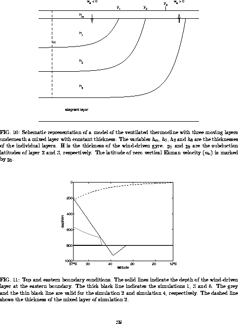
We chose the models of the ventilated thermocline by Luyten et al. (1983, hereafter LPS) and by Pedlosky and Robbins (1991, hereafter PR) for our numerical simulations. The PR model consists of three moving wind-driven layers beneath the mixed layer (Fig. 10). The water is assumed to be stagnant below the wind-driven circulation. The thickness of the mixed layer can be constant or latitude-dependent. The PR model becomes identical with the LPS model if the mixed layer thickness in the PR model is set to zero.

The parameters of the LPS model are the eastern boundary condition, the wind field, the subduction latitudes of layers 2 and 3 and the densities of the 4 layers. The PR model parameters are mainly the same as the parameters of the LPS model. Additional parameters are the mixed layer thickness and the density distribution in the mixed layer. The densities of layers 1 and 2 depend on the mixed layer density at the subduction latitudes of layers 2 and 3, respectively. The densities of layer 3 and layer 4 have to be prescribed.

The original models were adapted to the conditions on the southern hemisphere. Some limitations of the LPS model were relaxed. The introduction of a realistic coastline apparently leads to improved transport estimates. The eastern boundary may be open, allowing a more detailed interpretation of model results. The realistic coastline was also used in the PR model. When interpreting the results of the LPS/PR models one has to remember their limitations. These include (a) neglecting the thermohaline processes, (b) the large influence of the eastern boundary condition, and (c) the zonal alignment of the subduction latitudes.

The configurations of our simulations are presented in Table 8 and Fig.  11 . The subduction latitude of layer 3 (y₂) which represents the AAIW layer is set to 45^oS since the coldest SAMW sinks in the PFZ and thus feeds the AAIW. 40^oS is chosen as subduction latitude of layer 2 (y₁). The latitude of disappearing vertical Ekman velocity is marked by y₀. As an exception of this the subduction latitudes in simulation 3 are chosen to be at 40^oS and 35^oS for the layers 3 and 2, respectively. The densities are also inferred from hydrographic observations. The density of layer 3 was chosen such that it represents the AAIW layer with a mean density of 27.2 3 in the subtropics. The gyre depth at the eastern boundary is either set to 800 m or a latitude-dependent boundary condition is used. The thickness of the mixed layer for simulation 2 is obtained from an equation introduced by Pedlosky and Robbins (1991):

h$_m = a \times e^{-b \times (1-\varphi/y_{0e})}$

with
$\varphi$ = latitude,
y_0e = y₀ at the eastern boundary,
a = 3.8 m and
b = 160.

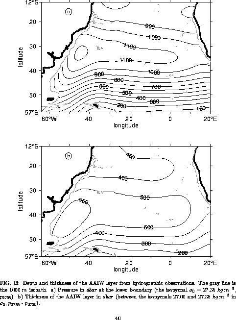
Case studies: It is known from observations that the maximum depth of the AAIW layer exceeds 1200 m near the shelf break of South America between 30^oS and 40^oS (Fig.  12 a). North of the gyre the depth decreases to less than 900 m. The thickness of the layer $\sigma _0$= (27 - 27.35) kg m³ increases from about 300 m at the southern rim of the gyre to more than 600 m in the gyre center and decreases again to less than 400 m at 20^oS (Fig. 12b).

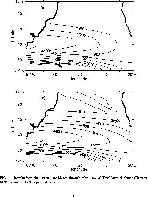
These features are qualitatively well reproduced in simulation 1, and the subtropical gyre can be seen clearly (Fig.  13 a). As in the observations the maximum depth (H) exceeds 1200 m in the center and decreases to less than 900 m farther north. The depth changes north of the subtropical gyre are weak as would be expected from observations, but the minima north of 20^oS are absent. The thickness of layer 3 (h₃) is also similar to observations, even though h₃ is larger than the observed thickness of the AAIW layer (compare Figs. 12b and 13b). This deviation can be explained as follows: South of 45^oS layer 3 represents the whole wind-driven water column, including the AAIW, since layers 1 and 2 do not exist. From there towards the north layer 3 is partitioned between the AAIW and the Central Water, and the partition of the AAIW increases towards the north. As in the observations the subtropical maximum of h₃ is mainly zonally oriented. But, in contrast to observations, the east-west gradient is quite large and the maximum is not enclosed by an isoline of elliptical shape. The 700 m isoline in Fig. 13b is broken in the northeastern basin because the models solution in the upwelling region near the African continent consists of complex numbers. Hence a vertical discretization is impossible there.

The deviations of simulation 1 from observed fields may have several reasons: First, the chosen model parameters, i. e. the boundary conditions, the subduction latitudes and the density stratification. Secondly, other physical processes not included in the model dynamics, i. e. the temporal variability, thermohaline processes and the western boundary current regime. Some of these aspects will be discussed briefly before the additional simulations are analyzed.

The maximum of H is located at 42^oS for the season presented in Fig. 13a. This latitude varies considerably from season to season and can be found much farther north (e. g. at 32^oS in austral winter 1993). The mean value of the gyre center latitude for all available seasonal ECMWF wind fields (austral autumn 1991 - austral spring 1993) is 39^oS. It is unlikely that the variability alone is a cause for the southward shift of the gyre center since 39^oS is still quite far south of the observed latitude of 33^oS (Fig. 12a).

The western boundary current system determines the longitudinal location of the maximum depth in the gyre center which is observed at 45^oW. At this longitude the maximum of H was located at 39^oS in austral autumn 1993, with the mean location for all available seasonal wind fields being 36^oS. This is still 3$^{\circ }$ farther south than one would expect from observations. It is likely that the overshooting of the western boundary currents in the Brazil/Malvinas Confluence Zone might also have an influence on the latitude of the gyre center. This effect, however, is expected to be small since it only affects the location of the SAC.

The effects of the density stratification are explained as follows. The model equations are based on density differences (reduced gravity) between adjacent layers. Reducing the densities of the upper 2 layers by 0.3 3 reduces the depth H in the ventilated zones north of y₂ by approximately 2%. The resulting transport changes in layer 3 are not significant (< 1%) because the gradient of H is nearly unchanged. A density change in layer 3 or 4 has a similar effect on H, but the influence on the transport is larger since the density difference between the two layers is multiplied by the gradient of H to estimate the velocity in layer 3. Decreasing the density of layer 4 by 0.1 3, which reduces the density difference between layer 3 and 4 by about 10%, can lower the transport in layer 3 by up to 10%. The effects of thermohaline processes will not be addressed here since the used models do not allow the introduction of an additional vertical velocity.

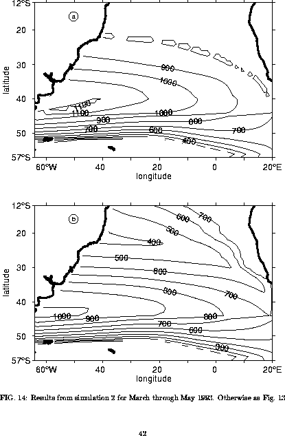
The simulation with a mixed layer (simulation 2, Fig.  14 ) results in a shallower subtropical gyre and a thinner third layer as in simulation 1. The isolines of H are more zonally aligned and a weak outflow through the eastern boundary can be seen. The latter is caused by the latitude-dependent mixed layer thickness (h_m, see Fig. 11, dashed line) which corresponds to an inflow that has to be compensated in the adjacent layer. The stronger eastward current is more realistic than the current in simulation 1. The thickness of layer 3 is also closer to observations than in simulation 1. In the northern model region the deviations are less than 100 m. The closed isolines of H at the northern edge of the ventilated zone and in the center of the subtropical gyre are caused by unstable solutions which depend on the choice of h_m. They do not affect the conclusions of the present analysis.

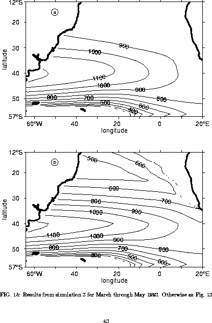
In simulation 3 the subduction latitudes y₁ and y₂ were shifted to the north by 5$^{\circ }$ (Fig.  15 ). The depth H is of course not affected by this change. The thickness of layer 3 is larger because the downward Ekman pumping acts on a larger area and the velocities are larger in some regions. As was discussed above the value of h₃ is overrated in simulation 1. Therefore the northward shift of the subduction latitudes leads to larger deviations between simulation and observation. A southward shift of the subduction latitudes would reduce this discrepancy. Such a southward shift, however, cannot be used in conjunction with all available seasonal wind fields. This can be understood if one considers the following. The model equations are based on the assumption that y₂ must be zonally aligned and that the east to west integrated vertical Ekman velocity must be negative at y₂ at all longitudes. For the shown season the latitude of zero vertical Ekman velocity ranges from 46^oS at 20^oW to 57^oS near the western and 52^oS at the eastern boundary. The zonally integrated vertical Ekman velocity would allow the choice of 47^oS as y₂. A simulation with this value for y₂ was not performed because this configuration can only be used for few of the available seasonal wind fields.

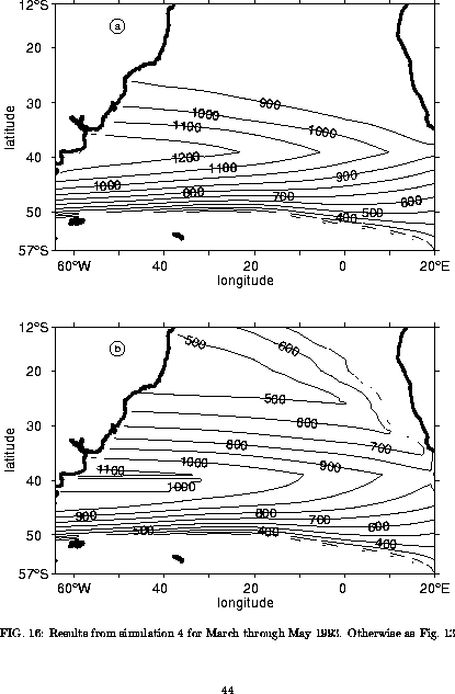
For simulation 4 an interoceanic exchange through the open eastern boundary was defined as follows. The transports were set to 5.3 Sv as inflow and 30 Sv as outflow. These values are smaller than the actual transport across 20^oE because the part related to the Agulhas Current retroflection west of this longitude and the corresponding flow into the Indian Ocean were not included. These transports are consistent with most of the available estimates from observations, e. g., the total inflow in the upper 1000 m is suggested to be 4 Sv by Garzoli and Gordon (1996) while Stramma and Peterson (1990) estimated 8 Sv. Both the outflowing and the inflowing currents were broadened to compensate for the models nature that a current through the eastern boundary flows strictly zonal through the whole basin. The resulting boundary condition is displayed in Fig. 11 (thin solid black line). North of 35^oS simulations 1 and 4 both lead to the same result since the eastern boundary condition is identical in this region (Figs.  16  and 13). In simulation 4 the gyre is deeper than in simulation 1 and H intersects the surface farther north. Therefore the eastward current is narrower and more zonal, which is more consistent with observations. The maxima of H and h₃ are farther north than in simulation 1 and the isolines of h₃ are more zonal in the eastern model region (Figs. 16b and 13b). The observed thickness of the AAIW layer has southeast to northwest oriented isolines in the eastward current. The 800 m line of h₃ has a similar orientation. In simulation 1 this isoline points from northwest to southeast. From simulation 4 one can conclude that the wind-driven gyre circulation together with the interoceanic exchange are well suited to describe the major features of the AAIW circulation in the subtropical South Atlantic.

It was shown that the geostrophic transport above the isopycnal$\sigma _0$= 27.35 3 can be explained by Sverdrup dynamics in good approximation. The deviations between the Sverdrup model and observations were addressed briefly. The simulations with the models of the ventilated thermocline allow a more detailed examination of the existing transport differences.

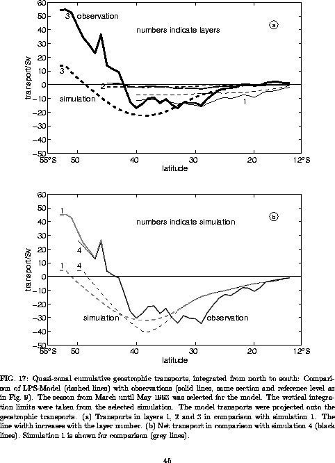
The cumulative transports for austral autumn 1993 of simulation 1 are compared with the geostrophic transport across the SAVE 5&6 section in Fig.  17 a. The vertical integration limits are taken from the presented simulation and the simulated transports are projected onto the resulting observed transports. The former takes care of the latitude dependent partition of layer 3 between AAIW and Central Water. The main features of the partition of the total transport among the three layers correspond to the observed transport distribution. However, the transports in layer 3 are excessive while they are underestimated in layers 1 and 2. These deviations from the observations are to be expected because the hydrographic section and the wind field originate from different times and because the interoceanic transport is neglected in the simulation. In layer 3 the transport in the westward branch of the subtropical gyre agrees quite well with the observations, but the current band is about 5$^{\circ }$ latitude broader than observed. In contrast the width of the eastward current agrees with the observations but its strength is underestimated by about 35 Sv. At 52$^{\circ }S$ the total difference between the observed and the simulated cumulative transport is 40 Sv, of which 2/3 can be attributed to the transport in the SAC between 43$^{\circ }S$ and 40$^{\circ }S$. The remaining deviation is due to the ACC and the higher westward transport in the simulations. The total simulated transport agrees better with observation. The deviation in the westward current is much smaller than in layer 3 while there is no significant change in the eastward current.

Opening the eastern boundary (simulation 4) reduces the deviations in the eastward current considerably from 35 Sv to 13 Sv of which again about 2/3 can be attributed to the SAC transport (Fig. 17b). At the same time the westward current is overestimated by about 5 Sv which is caused solely by the chosen inflow. We conclude that the discrepancies between simulation 1 and observations can, to some extent, be explained by the particular eastern boundary condition.

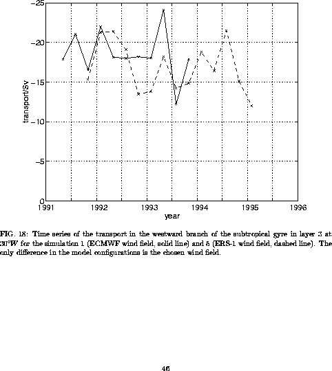
Seasonal variability: The westward transport in layer 3 at 30^oW varies between -12 Sv and -24 Sv for the ECMWF wind field (simulation 1, solid line in Fig.  18 ). The transport estimates based on the seasonal ERS-1 wind fields are mostly smaller (simulation 5, dashed line in Fig. 18), ranging from -12 Sv to -22 Sv. The means and standard deviations of the seasonal transports from simulations 1 and 5 are (-19$\pm$3) Sv and (-17$\pm$3) Sv, respectively. Both time series show a weak seasonality. The minima of the westward transport mostly occur in the second half of the year, sometimes the minimum extends into the beginning of the following year. Two aspects of the time series do not quite fit into this picture. First, simulation 1 does not have a clear minimum of the westward transport in 1992. Instead one can see a 1 year long period with low transports and a considerable deviation between simulations 1 and 5. Secondly, in austral summer 1995 the transport is smaller than in the previous season (simulation 1).

In the eastward current the layer 3 transport varies between 20 Sv and 44 Sv (simulation 1) and 13 Sv and 42 Sv (simulation 5). The corresponding means and standard deviations of the seasonal transports for simulations 1 and 5 are (36$\pm$7) Sv and (32$\pm$8) Sv, respectively. The observed eastward transport north of 49.5^oS can be larger by about a factor of 2 than the simulated transport. E. g. 24 Sv in austral autumn 1993 for simulation 1 versus 51 Sv across the SAVE 5&6 section. In the simulation with the open eastern boundary the deviation is reduced to less than 20%. E. g. 43 Sv in austral autumn 1993 for simulation 4 versus 49 Sv across the SAVE 5&6 section.

Seasonal transport changes are likely to be overestimated in a simple diagnostic model. In contrast to the real ocean, where it takes some time for a given wind field to change the circulation, the diagnostic model results in the equilibrium circulation for a given wind field.

We conclude that, taking the seasonal variability into account, about 90% of the observed westward and 50% of the observed eastward transport can be attributed to the circulation in the wind-driven subtropical gyre (simulations 1 and 5). The remaining transport deviations can partly be explained by the interoceanic exchange processes across the eastern boundary, even though the structure of the east- and westward currents still differs from observations (simulation 4).