The hydrographic data mainly consist of profiles from the National Oceanographic Data Center and a large number of profiles obtained during WOCE (sections A8 through A12, several repeat cruises in regions AR9 and AR15, and part of the METEOR 11/5 section, Roether et al., 1990).
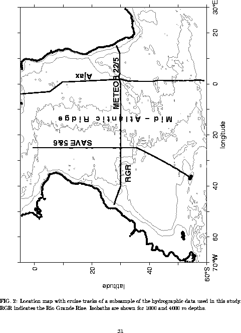
In cases where no high resolution profiles were available the data collected by Gouretzki and Jancke (1995) were used. The complete data set will be used to examine the AAIW layer in the South Atlantic. The hydrographic sections presented in Fig. 2 will be discussed more closely. The SAVE 5&6 sections (SAVE = South Atlantic Ventilation Experiment, Scripps Institution of Oceanography, 1992) were taken in February - April 1989. The WOCE section METEOR 22/5 (WOCE A10, Siedler et al., 1993) and the Ajax section (Rintoul, 1991) were performed in austral summer of 1993 and 1984, respectively.
The following Lagrangian current measurements are used: Data collected
during the ``Deep Basin Experiment'' (DBE, Hogg et al., 1996) by the Institut
für Meereskunde Kiel and during the ``Kap der Guten Hoffnung Experiment''
(KAPEX, Boebel et al., 1997a; Boebel et al., 1999c) by the Institut für
Meereskunde Kiel and the University of Cape Town as well as data provided
by the Scripps Institution of Oceanography (Davis et al., 1996). The Institut
für Meereskunde Kiel deployed neutrally buoyant RAFOS Floats (RAFOS
= SOFAR, ``Sound fixing and ranging'', spelled backwards; Rossby et al.,
1986) which were ballasted to reach equilibrium in the AAIW core layer.
Davis et al. (1996) used ALACE floats (ALACE = ``Autonomous LAgrangian
Current Explorer'') which were designed to measure currents at 750 m
depth. The initial depth of the ALACE floats ranged from 685 m to
815 m; during the missions depth changes of about ![]() 100
m
occurred.
100
m
occurred.
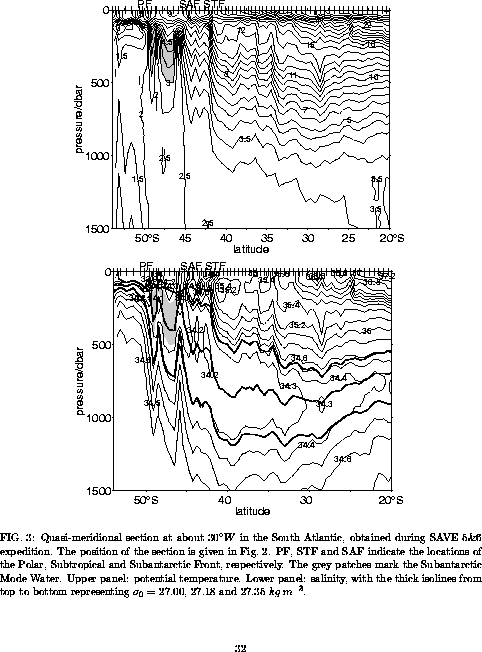
The salinity minimum of the AAIW and the northward salinity increase in this core layer can be seen clearly north of the SAF in Figs. 3 and 4 . South of the SAF, in the PFZ, the coldest SAMW, defined as the mode water with potential temperatures between 3oC and 4.5oC (e. g. McCartney, 1977), is indicated by grey patches. This SAMW is usually found in an about 300 m thick layer adjacent to the surface mixed layer and has been suggested to be an important source water of the AAIW (McCartney, 1977; Molinelli, 1981; Keffer, 1985). The observations indicate that the SAMW can be subducted at the SAF and feed fresher water into the AAIW layer in this case (Table 3 and Figs. 3 and 4). It will be shown later that subduction of SAMW indeed is an important process in the renewal of AAIW.
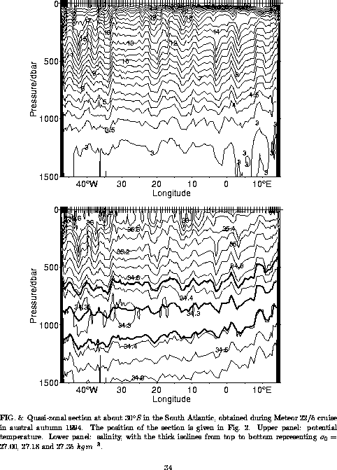
The three isopycnals (![]() = 27.00, 27.18 and 27.35 3) displayed in the salinity sections are a good
approximation for the upper boundary, the core and the lower boundary of
the AAIW layer in the subtropics and will be used throughout this study.
= 27.00, 27.18 and 27.35 3) displayed in the salinity sections are a good
approximation for the upper boundary, the core and the lower boundary of
the AAIW layer in the subtropics and will be used throughout this study.
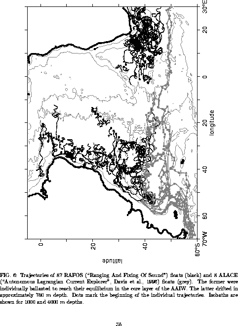
The water properties of the AAIW are nearly independent of the longitude when compared with the considerable northward increase of salinity and potential temperature (Figs. 3 , 4 and 5 ). The zonal section (Fig. 5), nonetheless shows an interesting feature, namely patches of low salinity water which are concentrated on the western side of the Mid-Atlantic Ridge (see Boebel et al., 1997b for more details). Three processes may cause this spatial variability: The meandering of a predominantly zonal current, a variable inflow of saltier AAIW from the Indian Ocean, or pulses of fresher AAIW flowing northward in the western South Atlantic. The latter could be caused by eddies from the Brazil-Malvinas Confluence Zone, by large meanders of the South Atlantic Current (SAC), or by a return current similar to the Brazil Return Current at the surface (Stramma, 1989; Rintoul, 1991). Float trajectories (Fig. 6 ) indicate that the water which flows into the Confluence Zone continues eastward in large meanders, or is caught in eddies that can cross the SAF to the north (not shown in detail). Both processes can inject fresher AAIW into the subtropical gyre (Boebel et al., 1999b; Schmid, 1998). The meanders can extend as far north as 35oS, where the Confluence eddies could also be observed. The trajectories do not show signs of a well-defined intermediate return current (Schmid, 1998). The meandering of the westward current of the subtropical gyre near the Rio Grande Rise has a similar signature as a return current in a zonal section (Boebel et al., 1997b).
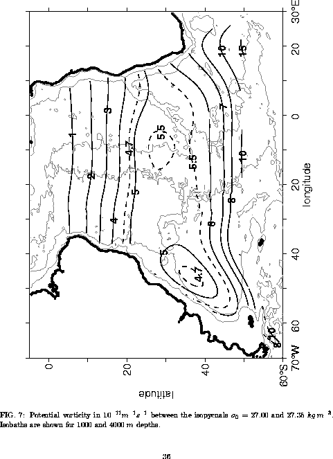
Potential vorticity can be used as a tracer for following the AAIW from
its sources through the South Atlantic. The potential vorticity of a water
parcel is conserved as long as no influence from the sea surface or mixing
with water of different potential vorticity occurs. We use ![]() for
the calculation of the potential vorticity (pv), where f
= Coriolis parameter,
for
the calculation of the potential vorticity (pv), where f
= Coriolis parameter, ![]() kg
m3,
kg
m3, ![]() = mean density of the layer defined by the isopycnals
= mean density of the layer defined by the isopycnals ![]() = 27.00 kg m3 and
= 27.00 kg m3 and ![]() = 27.35 kg m3, and
= 27.35 kg m3, and ![]() = thickness of the layer. The resulting distribution of potential vorticity
of the AAIW layer is shown in Fig. 7 . The
potential vorticity is relatively homogeneous in the subtropical South
Atlantic with a minimum in the west (<4.7 x 10⁻¹¹m-1s-1)
and a weak maximum near the Mid-Atlantic Ridge (>5.5 x 10⁻¹¹m-1s-1).
It is also apparent that the potential vorticity in the Agulhas Retroflection
region south of Africa is quite large (about 8 x 10-11m-1s-1)
while it is much lower in the Brazil-Malvinas Confluence Zone (about 5
x 10-11m-1s-1). These results
are consistent with Keffer's (1985) conclusion that the potential vorticity
maximum near the Mid-Atlantic Ridge can be traced back to the Agulhas region
and the Indian Ocean and that the lower potential vorticity south of this
maximum appears to be the coldest SAMW. The rather homogeneous potential
vorticity distribution in the gyre indicates that the recirculation dominates
the spreading of the AAIW, whereas the influence of the water inputs from
the Pacific and Indian Oceans is relatively small.
= thickness of the layer. The resulting distribution of potential vorticity
of the AAIW layer is shown in Fig. 7 . The
potential vorticity is relatively homogeneous in the subtropical South
Atlantic with a minimum in the west (<4.7 x 10⁻¹¹m-1s-1)
and a weak maximum near the Mid-Atlantic Ridge (>5.5 x 10⁻¹¹m-1s-1).
It is also apparent that the potential vorticity in the Agulhas Retroflection
region south of Africa is quite large (about 8 x 10-11m-1s-1)
while it is much lower in the Brazil-Malvinas Confluence Zone (about 5
x 10-11m-1s-1). These results
are consistent with Keffer's (1985) conclusion that the potential vorticity
maximum near the Mid-Atlantic Ridge can be traced back to the Agulhas region
and the Indian Ocean and that the lower potential vorticity south of this
maximum appears to be the coldest SAMW. The rather homogeneous potential
vorticity distribution in the gyre indicates that the recirculation dominates
the spreading of the AAIW, whereas the influence of the water inputs from
the Pacific and Indian Oceans is relatively small.
The isopycnal surface ![]() = 41.55 3 is used as a reference level for the geostrophic transport estimates
whenever possible (Tables 4a, 5a
and 6). This isopycnal is a good approximation
for a level of no motion since it is located between the North Atlantic
Deep Water and the Antarctic Bottom Water which are spreading in opposite
directions in large parts of the South Atlantic and since advection on
this isopycnal (below 3000 m) in the deep ocean can be expected
to be small in comparison with the velocities in the AAIW layer. The hydrographic
profiles taken during the Meteor 28/2 and the Polarstern ANT XII/2 cruises
were mostly terminated at 1500 dbar. This pressure level was used
as a reference level for these two sections. The underestimation of the
transport by this shallow reference level can be evaluated from a comparison
of the transports across the SAVE 5&6 section at 30oW. A
reference level at 1500 dbar yields a transport of 9 Sv,
whereas the deep reference level yields a transport of 16 Sv(Table
4a).
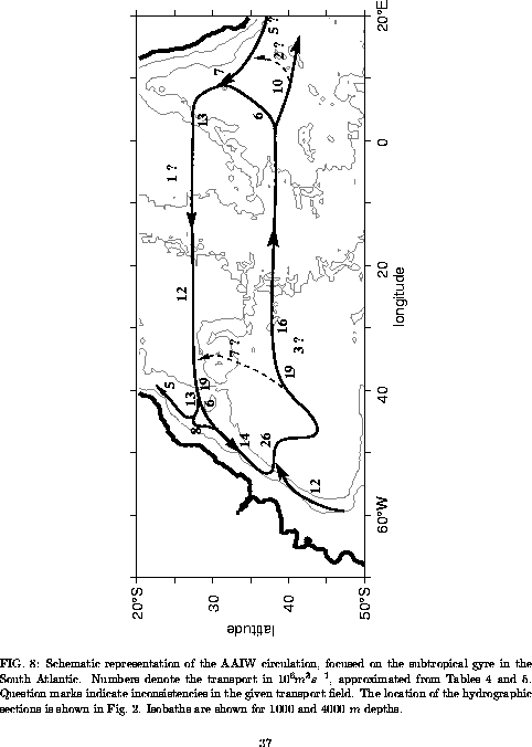
Only the geostrophic transports derived with the deep reference level were
included in Fig. 8 (for the location
of the sections see Fig. 2 ).
= 41.55 3 is used as a reference level for the geostrophic transport estimates
whenever possible (Tables 4a, 5a
and 6). This isopycnal is a good approximation
for a level of no motion since it is located between the North Atlantic
Deep Water and the Antarctic Bottom Water which are spreading in opposite
directions in large parts of the South Atlantic and since advection on
this isopycnal (below 3000 m) in the deep ocean can be expected
to be small in comparison with the velocities in the AAIW layer. The hydrographic
profiles taken during the Meteor 28/2 and the Polarstern ANT XII/2 cruises
were mostly terminated at 1500 dbar. This pressure level was used
as a reference level for these two sections. The underestimation of the
transport by this shallow reference level can be evaluated from a comparison
of the transports across the SAVE 5&6 section at 30oW. A
reference level at 1500 dbar yields a transport of 9 Sv,
whereas the deep reference level yields a transport of 16 Sv(Table
4a).
Only the geostrophic transports derived with the deep reference level were
included in Fig. 8 (for the location
of the sections see Fig. 2 ).
Our Lagrangian data were used to estimate mean velocities in 2![]() by 2
by 2![]() boxes. Lagrangian transport were derived from these velocities under the
assumption of a 500 m thick AAIW layer (Tables 4b
and 5b). This value was chosen since
it is a good compromise in the subtropics where the thickness of the AAIW
layer usually ranges from 400 m to 600 m. In the worst case,
a 100 m deviation from the used 500 mover the whole width
of the current, the transport error is 20%, because a constant velocity
over the whole layer is assumed. The agreement between the actual layer
thickness and the chosen 500 m is especially good in the westward
branch of the subtropical gyre, (490
boxes. Lagrangian transport were derived from these velocities under the
assumption of a 500 m thick AAIW layer (Tables 4b
and 5b). This value was chosen since
it is a good compromise in the subtropics where the thickness of the AAIW
layer usually ranges from 400 m to 600 m. In the worst case,
a 100 m deviation from the used 500 mover the whole width
of the current, the transport error is 20%, because a constant velocity
over the whole layer is assumed. The agreement between the actual layer
thickness and the chosen 500 m is especially good in the westward
branch of the subtropical gyre, (490![]() 50)
m,
while it is not quite as good in the SAC, (570
50)
m,
while it is not quite as good in the SAC, (570![]() 20)
m.
Thus the mean error introduced by our assumption is 2% for the transport
in the westward branch of the subtropical gyre and 14% in the SAC. The
latter seems quite large, but we think the uncertainty due to the high
variability in the confluence zone is currently the larger source for transport
errors.
20)
m.
Thus the mean error introduced by our assumption is 2% for the transport
in the westward branch of the subtropical gyre and 14% in the SAC. The
latter seems quite large, but we think the uncertainty due to the high
variability in the confluence zone is currently the larger source for transport
errors.
The eastward AAIW transports in the SAC range from 6 Sv to 26 Sv(Table 4 and Fig. 8). The geostrophic transport is largest near the western boundary with a rapid decrease from 26 Sv to 19 Sv between 52oW and about 41oW. Farther east both the Lagrangian and the geostrophic estimates indicate a slower decrease of the SAC transport from 19 Sv at 38oW to 16 Sv at 30oWand to 6 Sv at 1oE. The strong decrease between 30oW and 1oE suggests that the eastward flow leaves the subtropical gyre to the west of 1oE. The transports of the flow leaving/joining the subtropical gyre are chosen to close the budget. The transports to/from the Indian Ocean are hypothetical. In addition to the decrease of the SAC transport, a west to east decrease of the variability is clearly visible in the Lagrangian estimates (Table 4b).
The decrease of the South Atlantic Current by 3 Sv between 38oW and 30oW can be caused by an exchange between the South Atlantic Current and the Antarctic Circumpolar Current or it might be an artifact of the temporal variability of the flow. The former interpretation is partly supported by the ALACE trajectories (Fig. 6). These trajectories suggest an interaction of the Antarctic Circumpolar Current with the South Atlantic Current near 35oW and 20oW. In fact near 20oW the two currents seem to merge as one. Davis et al. (1996) noted this interaction problem in their analysis of the ALACE trajectories. The structure and the effects of the water exchange between the South Atlantic Current and the Antarctic Circumpolar Current remain unanswered questions.
The transport of 7 Sv from the South Atlantic Current to the north can be caused by mesoscale variability (see above). The fixed AAIW layer thickness given by the two density surfaces for the geostrophic transports and by a constant depth interval for the Lagrangian transports cannot be the only reason for the observed transport changes since the slackening of the South Atlantic Current transport is observed by both methods, and since the properties of the AAIW layer (temperature, salinity and thickness) are almost independent of longitude. The latter can be seen clearly when comparing the two sections at 30oW and 1oE in Figs. 3 and 4
The patterns of geostrophic transports in the westward branch of the
subtropical gyre suggest that they are almost independent of longitude
(Table 5 and Fig. 8).
The transport decrease of 1 Sv between 1oW and 25oW
is most likely caused by the temporal variability. Boebel et al. (1997b)
estimated a zonally averaged westward transport of (15![]() 5.4)
Sv
based on the first 15 RAFOS float trajectories (west of 27oW)
which is somewhat higher than the geostrophic transport at 25oW.
The increased amount of trajectories now available allows an estimation
of the zonal dependence of the transports in the western basin, revealing
a more complicated pattern. The transport actually increases between 30oW
and 36oW which might partly be caused by water of southern origin
(the 7 Svmentioned above) being fed into the westward flow. West
of 36oW the transport decreases again as the flow approaches
the western boundary. This is obviously due to the splitting of the current
into a northward and a southward branch in the Santos Bifurcation near
28oS adjacent to the western boundary (Boebel et al., 1997b
and 1999a). The transports at 36oW and 38oW seem
to be quite high (Table 5b). We think
that these high transports are due to a relatively poor data coverage.
Therefore we did not include these transports in the schematic presentation
in Fig. 8.
5.4)
Sv
based on the first 15 RAFOS float trajectories (west of 27oW)
which is somewhat higher than the geostrophic transport at 25oW.
The increased amount of trajectories now available allows an estimation
of the zonal dependence of the transports in the western basin, revealing
a more complicated pattern. The transport actually increases between 30oW
and 36oW which might partly be caused by water of southern origin
(the 7 Svmentioned above) being fed into the westward flow. West
of 36oW the transport decreases again as the flow approaches
the western boundary. This is obviously due to the splitting of the current
into a northward and a southward branch in the Santos Bifurcation near
28oS adjacent to the western boundary (Boebel et al., 1997b
and 1999a). The transports at 36oW and 38oW seem
to be quite high (Table 5b). We think
that these high transports are due to a relatively poor data coverage.
Therefore we did not include these transports in the schematic presentation
in Fig. 8.
The bifurcation can also be recognized in the transports along the western boundary which are shown in Table 6. The geostrophic transports are becoming larger with increasing distance from the Santos Bifurcation. This increase is especially obvious for the northward transport. The southward transport seems to be more variable. This is partly due to the varying length of the sections. The two sections with more than 10 Sv (Meteor 22/3 and Meteor 22/5) are reaching farther east while the other sections terminate very close to the eastern edge of the boundary current. The former sections have two bands of southward flow, the strong boundary current and somewhat weaker flow directly offshore of the boundary current. The transport in the boundary current is between 5 Sv and 6 Svfor both sections. The transports presented in Table 6 show that the northward transport is smaller than the southward transport, nearly 3/4 of the 19 Sv at 40oW recirculate in the subtropical gyre, and about 1/4 flows north along the western boundary (Schmid, 1998).