THREE-DIMENSIONAL VARIATIONAL ANALYSIS OF AIRBORNE DOPPLER OBSERVATIONS
Principal Investigator:
John F. Gamache
Collaborating Scientist: Wen-Chau Lee/NCAR/ATD/RSF
Objective: To improve dual- and multiple-Doppler
analyses by incorporating the Doppler projection equations, the three-dimensional
continuity equation, and filtering within a variational scheme.
Rationale: The solution of a Doppler wind analysis
involves two or more projection equations, and one continuity equation.
The solution of these three together is difficult. In the past, the vertical
wind was first assumed to be zero and then the projection equations were
solved for the horizontal wind components. The divergence of the horizontal
components was then integrated to determine the vertical wind. The new
vertical wind was then used in the projection equations to determine a
new horizontal wind field. This process was to be iterated to a solution.
The process was unstable for Doppler radials more than approximately 45
degrees from horizontal. Thus these data must be thrown out if the process
is to be iterated to a convergent solution. Throwing all three equations
into a cost function, however, allows all three equations to be solved
simultaneously, and thus Doppler radials above 45 degrees may be kept in
the analysis. This is because the continuity equation is also solved in
all three directions, and not just in the vertical. Another advantage is
that since the filtering is included in the cost function at a much lower
cost than continuity, a smoother wind field is found that still satisfies
the continuity equation closely.
Method: Several steps are required in determining
wind field from dual- or multiple-Doppler observations
-
Doppler data are first interpolated to a three-dimensional grid.
-
The cost function may then be determined for the difference between the
projection of the solution motion of the precipitation back on to the Doppler
radial and the measured Doppler radial velocity.
-
Next a grid point representation of the anelastic three dimensional divergence
is determined. The cost function for the difference between that divergence
and zero is determined.
-
Similarly, a simple equation that says that the value of six times the
density weighted wind component at a point is equal to the sum of the density
weighted wind component at the surrounding six points. The difference between
the weighted sum of those seven solution variables and zero is also added
to the cost function.
-
A bottom boundary condition of zero vertical wind is also imposed within
the cost function.
-
Represent the cost function as a matrix equation with several bands. The
matrix is symmetric positive definite and the matrix equation is solved
by the conjugate gradient method.
Accomplishments in FY97: The past year has seen
some exciting developments in the analysis
-
The option to incorporate a top boundary condition of zero vertical wind
approximately 1 km above echo top, where echo top is defined as the highest
level in a column where two independent Doppler observations are found.
-
A subroutine was written to detect those regions of the analysis that were
not properly bounded, so the option is there to remove them
-
Synthetic wind fields were devised and used to test the analysis method.
New insights in how the analysis actually handles difficult wind fields
were found. The synthetic fields also showed that a complicated wind
field can be represented fairly well by the technique, but not when errors
are introduced. Thus the major culprit in the analysis method is
data collection and interpolation. Errors of this sort can introduce
high-frequency errors that are aliased by the grid point solution.
-
A fourier-component analysis for the azimuthal direction around a storm
center was introduced into the method. This permits a analysis similar
to the VTD analysis; however, flat-plane scanning through storm center
is not required.
-
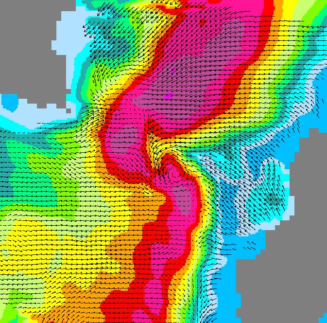
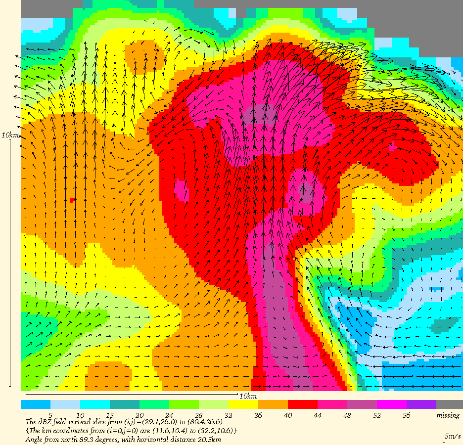
Data from the 1995 VORTEX experiment, on 7 May 1995, have been analyzed
with this method and a horizontal and vertical slice through the analysis
are shown in Figs. 1 and 2,
respectively.
Go to Project 97 page.
Last modified: 11/13/97