![]()
![]()
The ENSO-CLIPER model was constructed from a dependent data set of 43 years which, given the typical ENSO timescale of three to five years giving ten to fifteen complete ENSO realizations, may be on the short side of time length needed for this regression technique. Other SST data sets were examined before selecting the Smith et. al. (1996) data. However, it was found that before approximately 1950 the equatorial Pacific region data quality was inadequate for the purposes of this scheme. Included in the earlier section are estimates of future skill based on the work of Davis and Shapiro, but it is unknown whether these estimates will hold true in completely independent data. To supplement the reduced correlation and RMSE values, the available independent forecast values since 1993 and their verification are listed in Appendix A and a comparison is performed versus other published schemes over that same period.
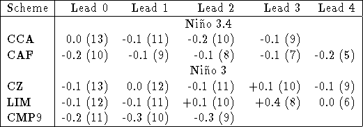
Overall, the years 1993-96 have been a particularly difficult time period of ENSO history to predict, because of the long running 1990-95 warm ENSO conditions. Using data available in the ELLFB (Barnston 1993, 1994, 1995, 1996) as both numeric and graphical format, forecasts of Niño 3.4 (CCA and CAF) and Nino 3 (CZ, LIM, CMP9) over the same years but with differing initial forecast times, seasonal leads and verification times are compared. Table 3 shows the RMSE differences between the ENSO-CLIPER minus the various schemes listed above. Note that with only a couple exceptions, the ENSO-CLIPER outperformed (shown as a negative difference) or was equivalent to its competitors. Only LIM - another statistically based model, significantly improved upon ENSO-CLIPER, and this only occurred at a single (three seasons) lead time.

Table 3: RMSE differences produced by taking ENSO-CLIPER
based RMSE minus the RMSE of the various schemes listed in the first
column. Negative numbers indicate that the ENSO-CLIPER scheme
outperformed the methodology listed at the left. Note that the
verification times varied between individual
schemes. The number of available comparisons per lead time and
methodology is shown in the parenthesis.
Similarly, one could calculate the linear correlation coefficients between the observed and predicted values for the five schemes listed above and the ENSO-CLIPER. These results, shown in Table 4, suggest again that no statistical scheme or numerical model have had success improving over the ENSO-CLIPER scheme. It is also apparent that all of the schemes - ENSO-CLIPER included - have been unable to make independent forecasts that provide a non-negligible, positive amount of the variance explained beyond lead one. Granted these results are based upon a very small sample, but all are independent and all are fairly judged against one another.

Table 4: Correlation coefficients (X 100) between various schemes,
ENSO-CLIPER and the observed SST anomalies for the same periods
discussed in Table 3. The ``Mod'' column indicates the correlations of the
various models listed to the left versus the observed SST anomalies
and the ``EC'' column indicates the correlation values for the same time
periods using ENSO-CLIPER.
Again the difficulties that all of these models have been having stems, at least to some degree, to the rather anomalous long warm event (1990-95) that occurred during the years under consideration. However, it appears with the limited testing shown here that 1) ENSO-CLIPER is at least competitive with many of the currently available models; 2) none of the intercompared models during the years 1993-96 showed ``skill" in forecaster ENSO as defined as significantly exceed the forecasting ability of ENSO-CLIPER (with the possible exception of lead three LIM); and 3) all models including ENSO-CLIPER performed poorly during 1993-96.
![]()