* Corresponding author address:
Dr. Paul W. Mielke Jr., Department of Statistics, Colorado State University, Fort Collins, CO 80523.
E-mail: mielke@lamar.colostate.edu

AMS Copyright Notice © Copyright 1997 American Meteorological Society (AMS). Permission to use figures, tables, and brief excerpts from this work in scientific and educational works is hereby granted provided that the source is acknowledged. Any use of material in this work that is determined to be "fair use" under Section 107 or that satisfies the conditions specified in Section 108 of the U.S. Copyright Law (17 USC, as revised by P.L. 94-553) does not require the Society's permission. Republication, systematic reproduction, posting in electronic form on servers, or other uses of this material, except as exempted by the above statements, requires written permission or license from the AMS. Additional details are provided in the AMS Copyright Policies, available from the AMS at 617-227-2425 or amspubs@ametsoc.org. Permission to place a copy of this work on this server has been provided by the AMS. The AMS does not guarantee that the copy provided here is an accurate copy of the published work.
 

ABSTRACT
The results of a simulation study of multiple regression prediction models for meteorological forecasting are reported. The effects of sample size, amount, and severity of nonrepresentative data in the population, inclusion of noninformative predictors, and least (sum of) absolute deviations (LAD) and least (sum of) squared deviations (LSD) regression models are examined on five populations constructed from meteorological data. Artificial skill is shown to be a product of small sample size, LSD regression, and nonrepresentative data. Validation of sample results is examined, and LAD regression is found to be superior to LSD regression when sample size is small and nonrepresentative data are present.

 1. Introduction

Recently developed prediction models of various atmospheric phenomena have motivated this study (Gray et al. 1992, 1993, 1994) . We are interested in the influence of various conditions on the degree of agreement between observed values and values predicted by a meteorological regression model. Of particular interest are differences between least (sum of) absolute deviations LAD) regression models and least (sum of)squared deviations (LSD) regression models (commonly termed least squares models) under a variety of research conditions. Such conditions include sample size, the inclusion of uninformative independent variables, and the influence of the amount and severity of nonrepresentative data.

In the context of artificial skill and validation in meteorological forecasting, we present examples of prediction of intensity change of Atlantic tropical cyclones 24 h into the future. Datasets containing values of independent variables that deviate either moderately or severely from the bulk of the available data are termed "nonrepresentative" or "contaminated" datasets. The use of contaminated data is to represent potential situations that frequently arise in forecasting, whether it be day-to-day or seasonal forecasting. For predictions of tropical cyclone intensity change in this case,large errors (or contamination ) in the predictors can frequently occur. One common problem relates to monitoring tropical cyclones at night with only infrared-channel satellite data available. When strong vertical shear develops, often the convectively active portion of the storm can be separated from the lower portion of the storm circulation. At night, with just the infrared pictures, a shear-forced separation will not be detectable because the lower portion of the storm will be nearly invisible to the infrared sensors. When the first visible channel images are available in the morning and it becomes apparent that the storm has been sheared, there would have been overnight errors of current intensity by up to 15 m s^-1 too high, position errors about 100 km or more, and several meters per second in storm motion error (Holland 1993) . Real errors like this are similar to the type of contamination that we have built into the skill testing.

The results of this study suggest that large samples ( i.e., n > 100) are needed for most forecasting studies of this type and that LAD regression is superior to LSD regression whenever a small amount of moderately contaminated data is present. The results also suggest that meteorological regression studies of the type considered here should not be undertaken whenever
a large amount of severely contaminated data is expected.
 

2. Description of statistical measures

Let the population and sample sizes be denoted by N and n, respectively; let y_i denote the dependent (predicted)variable; and let x_il, . . . , x_ip denote the p independent (predictor) variables associated with the ith of n events. Consider the linear regression model given by
 
 

where β₀, . . . , β_p are p + 1 unknown parameters and e_i is an error term associated with the ith of n events. The LAD and LSD prediction equations are given by

where  _i is the predicted value of y_i and o. . . ., p minimize the expression

and where v = 1 and v = 2 are associated with the LAD and LSD regression models, respectively.

The question arises as how best to determine the correspondence between the observed (y_i ) values and the predicted ( ) values, for i = 1,..., n . A widely used method is to calculate the Pearson product-moment correlation coefficient (r) or the coefficient of determination (r² ) between the paired values ( e.g., Barnston and Van den Dool 1993) . The coefficient of determination is strictly a measure of linearity, and r² = 1.0 implies that all paired values of y_i and _i for i = 1,..., n fall on a line that does not necessarily have a unit slope nor passes though the origin.

Consequently, an r² 1.0 does not imply complete agreement between the paired y_i and _i values since r² = 1.0 if y_i and  differ by an additive constant and/or by a multiplicative constant. For example, if the observed values are y_i = i for i = 1,... n and the corresponding predicted values are  = 50 + 2i for i = 1,...n, then the coefficient of determination between y_i and  is r² = 1.0; clearly, the prediction model that generated the _i values is useless. Thus, the use of the Pearson product-moment correlation coefficient in assessing prediction accuracy often produces an inflated index of forecast skill. To avoid this problem, either the mean square error (MSE) given by

or the root-mean-square error (rmse) given by

is often employed. While the MSE and rmse are zero when the y_i and i values are identical, the two measures are not standardized measures and have no upper limits. In addition, neither measure is independent of the unit of measurement, and therefore, the measures are difficult to compare across studies. For example, if y_i is measured first in knots and second in meters per second, the values of the MSE and the rmse will change. Finally, both the MSE and rmse are conceptually misleading. The often-cited geometric representation of row vectors (y₁, . . . , y_n) and ( ₁, . . . , _n) in an n-dimensional space and the interpretation of n^1/2 rmse as the Euclidean distance between the observed and predicted n-dimensional points in this space is an artificial construct. In reality, the n paired values {(y₁ , ₁), . . . . , (y_n, _n)} are n repeated pairs of points in a one-dimensional space. Furthermore, the MSE and the rmse involve squared Euclidean differences and they can be heavily influenced by one or more extreme values (Cotton et al. 1994) , which are not uncommon in meteorological research. An alternative to the MSE or the rmse is the mean absolute error (MAE) , in which the absolute differences are considered; that is,
 
 

Like the MSE and the rmse, the MAE is not independent of the unit of measurement, is not a standardized measure, and has no upper limit. However, the MAE does mitigate the problem of extreme values. Finally, while the rmse is a minimum when the _i values are based on an LSD prediction model, the MAE is a minimum when the _i values are based on an LAD prediction
model. Although the MAE is often computed on an LSD prediction model ( e.g., Elsner and Schmertmann 1994) , it is difficult to interpret when based on LSD regression, and when LSD regression is used, MAE values may not be comparable.

Because of the problems with these measures, many researchers have turned to measures of agreement in assessing prediction accuracy for example, Willmott(1982) , Willmott et al.(1985) , Tucker et al. (1989) ,Gray et al. (1992) , McCabe and Legates (1992) , Badescu(1993) , Elsner and Schmertmann (1993) , Hess and Elsner (1994) , and Cotton et al. (1994) . For a recent comparison of various measures of agreement, see Watterson (1996) .

In this study, the measure of agreement for both the LAD and LSD prediction equations is given by

where

v = 1 is associated with LAD regression, v = 2 is associated with LSD regression, and µ  is the average value of  over all n! equally likely permutations of y₁ , . . . , y_n relative to ₁, . . . , _n under the null hypothesis that the n pairs (y_i and _i for i = 1, .... n) are merely the result of random assignment. This reduces to the simple computational form given by

Since  is a chance-corrected measure of agreement,  = 1.0 implies that all paired values of y_i and _i for i = 1,..., n fall on a line with unit slope that passes through the origin ( i.e., a perfect forecast) . Because  = MAE when v = 1 and  = MSE when v = 2, all values of  are based on v = 1 due to the geometric concern involving mse.
 

3. Construction of the population

In the notation of the previous section, the 3958 available primary events used to construct the five populations of this study consist of a dependent (predicted) variable (y) and 10 independent (predictor) variables (x₁, . . . , x_p), where p = 10. The dependent "variable" for these populations is constructed from two datasets. In one dataset the predicted values are intensity change 24 h into the future; in the second dataset, the predicted values are intensity 24 h into the future. A simulation study of this type requires a population with a  value of approximately 0.50 in order to observe changes due to various sampling conditions and to reflect obtained  values in related studies (Gray et al. 1992, 1993, 1994). The descriptions for each of these variables follow:

y Intensity change/ intensity 24 h into the future ( in knots)
x₁ Julian date ( e.g., 1 is 1 January and 365 is 31December)
x₂ Latitude ( in degrees and tenths of degrees)
x₃ Longitude ( in degrees and tenths of degrees)
x₄ Current intensity ( in knots)
x₅ Change of intensity in last 12 h (in knots)
x₆ Change of intensity in last 24 h (in knots)
x₇ Speed of storm in zonal direction ( in knots, wherepositive is toward the east)
x₈ Speed of storm in meridional direction ( in knots,where positive is toward the north)
x₉ Absolute magnitude of speed of storm ( in knots)
x₁₀ Potential intensity difference ( in knots) is based

upon an exponential function of sea surface temperature (SST) minus the current intensity (DeMaria and Kaplan 1994)

The intensity change values and the 10 predictors were obtained from two separate datasets. Most of the values were constructed from the Atlantic basin best track data maintained by the National Hurricane Center (Jarvinen et al. 1984) . Tropical storm and hurricane statistics of position, highest surface sustained winds, and lowest surface pressure ( if measured) for every 6 h of their existence are available. Tropical storm data were removed for those storms that became extratropical or weakened below 35 kt by the 24-h verification time.Additionally, the SST data were obtained from the monthly SST (COADS) climatology (Reynolds 1988). These data are available on a 2º x 2º grid based on the period 1950-79.

Two regression models designated as case 10 and case 6 are examined in this study. Case 10 involves all 10 independent variables (p = 10), whereas case 6 involves only 6 of the 10 independent variables ( variables x₆ , x₇ , x₈ , and x₉ are removed and p = 6). All datasets used in this study are available from the authors.

4. Simulation procedures

The present study investigates the effect of sample size, type of regression model (LAD and LSD) , amount and degree of contamination, and noise-to-signal ratio on the degree of agreement between observed and predicted values in five populations that differ in amount and degree of contaminated data. Sample sizes (n) of 15, 25, 40, 65, 100, 160, 250, and 500 events are obtained from a fixed population of N = 3958 events that, for the purpose of this study, is not contaminated with extreme cases, a fixed population of N = 3998 events consisting of the initial population and 40 moderately extreme events (1% moderate contamination), a fixed population of N = 3998 events consisting of the initial population and 40 very extreme events (1% severe contamination) , a fixed population of N = 4158 events consisting of the initial population and 200 moderately extreme events (5% moderate contamination), and a fixed population of N = 4158 events consisting of the initial population and 200 very extreme events (5% severe contamination) .

The moderate 1% (5%) contamination consists of 40 (200) carefully designed additional events. The additional values of the independent variables were selected from the lowest and highest values of the specified independent variable in the initial population. Then, either the lowest or the highest value was selected, based on a random binary choice. The associated values of the dependent variable were selected from the center of the distribution of the dependent variable in the initial population, near the median. The severe 1% (5%) contamination involves 40 (200) centered dependent-variable values with the values of the independent variables placed at 2.5 times the lower and upper values of the ranges associated with the corresponding independent variables in the initial population. The random sampling of events from each population was implemented in the bootstrap context; that is, the random sampling was accomplished with replacement. It should be noted that the contamination and examination of datasets containing extreme values is not new. Michaelsen (1987) analyzed datasets containing
naturally occurring extreme values. Barnston and Van den Dool 1993 contaminated Gaussian datasets with extreme values in a study of cross-validated skill. As Barnston and Van den Dool (1993) note, extreme values are representative of many meteorological events and, in addition, inclusion of very extreme values, up to 10 standard deviations from the mean    (Barnston and Van den Dool 1993) , may be important as "extreme design experiments." Finally, it should be emphasized that the initial population was designed and constructed from real data. The added events that contaminate the initial population create populations of data that are contaminated relative to the initial population. Whatever contamination preexists in the initial
population of real data is unknown.

Two prediction models are considered for each population. The first prediction model (case 10) consists of p = 10 independent variables, and the second prediction model (case 6) consists of p = 6 independent variables. In case 10, 4 of the 10 independent variables were found to contribute no information to the predictions. Case 6 is merely the prediction model with the four noncontributing independent variables of case 10 deleted. Beginning with the 10 independent variables of case 10, backward selection was used on the entire population to identify the 6 contributing independent variables of case 6. The reason for the two prediction models is to examine the effect of including noncontributing independent variables in a prediction model.

A few caveats regarding the simulation study and its application to actual meteorological research follow. 1) Although the initial population is constructed from actual meteorological data, the purpose of this study is not to generate prediction models but rather to investigate statistical questions involving meteorological prediction methods. 2) While this study depends on the five specific populations that have been generated, the findings of this study are anticipated to hold for a variety of other populations. 3) Since this study involves random sampling from a fixed population, the results must be interpreted as a stationary process rather than an evolutionary process, which is commonly associated with climatic events in a time series framework. 4) In practice an investigator often exhausts the available data associated with a given study. Consequently, the results of the present study should be interpreted in the context of an unknown population for which a prediction model is desired. 5) The present study is strictly an empirical study. No distributional assumptions (e.g.,normality) are made about any of the variables in the population. 6) The purpose of this study is to help investigators choose sample sizes and regression techniques for future research. Because of the artificial nature of the dependent variable, no predictions to actual
meteorological events are intended.
 

5. Discussion of the findings

The findings of the study are summarized in Tables 1, 2, 3, 4, 5. In Tables 1a, 2a, 3a, 4a, and 5a, each row is specified by 1) a sample size (n), 2) p = 10 (case 10) and p = 6 (case 6) independent variables, and 3) LAD and LSD regression analyses. In each of these tables the first column (C1) contains the true  values for the designated population, the second column (C2) contains
the average of 10 000 randomly obtained sample  values of a specified size where the  values are based on the true population regression coefficients, and the third column (C3) contains the average of 10 000 randomly obtained sample  values where the  values are based on the sample regression coefficients for each of the 10 000 independent samples. The fourth column(C4) is more complicated and is designed to measure the effectiveness of validating sample regression coefficients. Here the sample regression coefficients from 10 000 random samples are obtained from column C3; then, for each of these 10 000 sets of sample regression coefficients an additional set of five independent random samples of the same designated size (n = 15, ...500) are drawn from the population. The sample regression coefficients from C3 are then applied to each of these five new samples, and  values are computed for each of these five samples for a total of 50 000  values. The average of these 50 000  values is reported in column C4 of Table 1a, yielding a measure of the effectiveness of sample validation - that is, applying the sample regression coefficients from a single sample to five new independent samples drawn from the same population.
 

In Tables 1b, 2b, 3b, 4b, and 5b, each row is specified by a sample size (n), p = 10 (case 10) and  p = 6 (case 6) independent variables, and LAD and LSD regression analyses. In each of these tables the first column(C2/C1) contains the ratio of the average  value of C2 to the corresponding true population  value of C1, the second column (C3/C1) contains the ratio of the average  value of C3 to the corresponding true population  value of C1, the third column (C4/C1) contains the ratio of the average  value of C4 to the corresponding true population  value of C1, and the fourth column (C4/C3) contains the ratio of the average  value of C4 to the average  value of C3.
 

a. Overview of the findings

There are four types of predictive skill to be examined in this study: true skill, optimal skill, artificial skill, and expected skill. Each of the four types is considered under the following conditions: contamination of the population data in both degree and amount; type of regression model used, that is, LAD and LSD; the ratio of noise-to-signal in the data where the 10-predictor model (case 10) contains a relatively high noise-tosignal ratio and the 6-predictor model (case 6) contains a relatively low noise-to-signal ratio; and sample size, which varies from n = 15 to n = 500.

The first type of skill to be considered is true skill, which is defined as the agreement, measured by a value, between the observed (y) and predicted ( ) values when the entire population is available and the  values are based on the true population regression coefficients. In general, true skill is used as a benchmark against which the other three forms of skill are evaluated. The true skill  values are given in column C1 of Tables 1a, 2a, 3a, 4a, and 5a.

The second type of skill is optimal skill, which reflects the average agreement, measured by a value,  between the observed (y) and predicted ( ) values when only a specified sample is available and the  values are based on the true population regression coefficients. Optimal skill is measured as the ratio of the sample  value, with the population regression coefficients presumed known, to the corresponding true skill  value. Specifically, the relevant values are given in  column C2 of Tables 1a, 2a, 3a, 4a, and 5a, and the optimal skill ratios are given in the C2/C1 column of Tables 1b, 2b, 3b, 4b, and 5b. The expectation is that the tabled C2/C1 ratios will be a little less than 1.0, even for small samples, because they reflect what would happen if a researcher drew a sample and, fortuitously, happened to get a set of sample-based regression coefficients very close to the true population regression coefficients. The reason that the tabled C2/ C1 ratios are not equal to 1.0 is because the sum of errors in the sample is not minimized by the population regression coefficients. Note, however, that as sample size increases the corresponding sample optimal fit approaches the population fit and the C2/C1 values approach 1.0.

The third type of skill is artificial skill, which reflects the average agreement, measured by a  value, between the observed (y) and predicted ( ) values when a specified sample is available and the  values are based on the sample regression coefficients (Shapiro 1984) . For an alternative definition of artificial skill, based on the difference between hindcast and forecast skill, see Michaelsen (1987) . Artificial skill is measured as the ratio of the sample  value, with the population regression coefficients presumed unknown, to the corresponding true skill  value. Specifically, the relevant  values are given in column C3 of Tables 1a, 2a, 3a, 4a, and 5a, and the artificial skill ratios are given in the C3/C1 column of Tables 1b, 2b, 3b, 4b, and 5b. The expectation is that the C3/C1 values will be slightly above 1.0 because of what is commonly termed "retrospective"
fit (Copas 1983) between the y and  values; that is, the sum of errors is minimized because the regression coefficients are based on the sample data. In general, tabled C3/C1 values greater than 1.0 reflect the amount of artificial skill inherent in retrospective fit; for convenience, we will call this a "degrading" of the prediction; that is, the sample-based  value overestimates the true population  value and the sample  value must be degraded by multiplying it by the reciprocal of the tabled C3/C1 value.

It should be noted in this context that artificial skill is a type of optimizing bias where the results are biased upward. There is a second type of bias that also contributes to artificial skill: selection bias. This occurs when a subset of independent variables is selected from the population based on information in the sample. As in the case of optimizing bias,artificial skill is biased upward when selection bias is present. In this study, the measure of artificial skill reflects only optimizing bias. Selection bias has been controlled by selecting the two sets of independent variables (cases 10 and 6) from information contained in the designed population, not from information contained in a sample.

The fourth type of skill is expected skill, which reflects the average agreement, measured by a  value, between the observed (y) and predicted () values when a specified sample is available and the sample regression coefficients are applied to an additional set of samples independently drawn from the same population. Expected skill is measured as the ratio of the average sample  value to the corresponding true skill  value. The relevant  values are given in column C4 Pr of Tables 1a, 2a, 3a, 4a, and 5a, and the expected skill ratios are given in the C4/C1 column of Tables 1b, 2b, 3b, 4b, and 5b. The expectation is that the tabled C4/C1 values will be slightly less than 1.0 because they reflect what is commonly termed "prospective" or "validation" fit (Copas 1983) between the y and  values; that is, the sum of errors is not minimized because the regression coefficients are based on only one of the six independently drawn random samples. In general, tabled C4/C1 values less than 1.0 indicate the amount of skill that is expected relative to the true skill possible when a population is available.More specifically, if researchers were to use the sample coefficients in a prediction equation, as is commonly done in practice, then the C4/C1 values indicate the expected reduction in fit of the y and  values for future results. Any tabled C4/C1 value greater than 1.0 is cause for concern since this indicates that the sample estimates of the population regression coefficients provide a better validation fit, on average, than would be possible had the actual population been available and is evidence that some sort of inflation of expected skill is present in the analysis.
 

b. Population 1

Population 1 is the initial population of N = 3958 noncontaminated events. The results of the analysis of population 1 are summarized in Tables 1a and 1b. Since sample  values that are based on true population regression coefficients behave very much like unbiased estimators of the true  values, the average sample  values in column C2 of Table 1a are, as expected, very close to the true population  values in column C1 of Table 1a. The corresponding ratios are given in the C2/ C1 column of Table 1b. It is obvious from an inspection of these values that larger sample sizes provide better predictions; that is, the ratio approaches 1.0 as sample size increases from n = 15 to n = 500, there are no differences between the 10-predictor model (case 10) and the 6-predictor model   (case 6) , and there are no appreciable differences between the LAD and LSD regression models, other conditions being equal.
 

In most studies, the population regression coefficients are not known, and the sample value is based  strictly on the sample regression coefficients, as in column C3 of Table 1a. Whenever a sample is obtained from a population there will be, on average, a degrading of the prediction; that is, the sample-based  value will overestimate the true population  value. Column C3/C1 in Table 1b is a measure of the degrading for this population. Inspection of the C3/C1 column indicates that the sample  values are indeed biased upward, as all of the C3/C1 values are greater than 1.0.
 

It is also clear that the amount of degrading decreases with increasing sample size, that case 6 (6 predictors)is superior to case 10 (10 predictors) , and that the LSD regression model provides less bias than the LAD regression model. Note also that most of these differences disappear as the sample size becomes larger.

A comparison of the C2/C1 and C3/C1 columns yields an important conclusion: should an investigator be fortunate enough to select a sample, of any size, that yields regression coefficients that are close to the true population regression coefficients, then, as can be seen in column C2/C1, the predicted values will show high agreement with the observed values. A luxury of a simulationstudy of this type is that the true population values are known. In most research situations, an investigator has only a single sample with which to work and has no way of knowing if the obtained value is  too high.
 

The problem of validated predictions ( really predictions which are not validated) is important in meteorological forecasting, and the C4/C1 column provides a measure of the effectiveness of validated predictions for population 1. The values presented in the C4/C1 column indicate that validation is extremely poor for small sample sizes where the expected skill ratios are considerably less than 1.0, but the problem nearly disappears for larger samples. There is a considerable differencebetween case 10 and case 6 for small samples,but most of the difference disappears for the larger samples.The LSD regression model is superior to the LAD regression model for small samples, but there is no difference for the larger samples. Note that no tabled C4/C1 value exceeds 1.0. Values greater than 1.0 would indicate, as noted previously, that sample estimates of the population regression coefficients provide better validation fits, on average, than would be possible had the actual population been available. The ratio values in the C4/C3 column contain the amount of expected skill (C4/C1) adjusted for the amount of artificial skill (C3/C1) . There is an amount by which validation fit (C4) falls short of retrospective fit (C3), and the values in the C4/C3 column summarize this "shrinkage" ( cf. Copas 1983) in a ratio format. The C4/C3 ratio provides the most stringent measure of anticipated reduction in prediction, relative to available sample information.
While it is not possible to compare across cases (10 and 6) or across models (LAD and LSD) because a common base does not exist, it is possible to compare across sample size (n = 15 to n =500) within the same case and model. It is clear that, within these restrictions,larger sample sizes yield less shrinkage of expected skill than smaller sample sizes. For example, given case 6, the LAD regression model, and n = 15, C4/C3 = 0.461; however, C4/C3 = 0.762 when n = 40. Shrinkage in expected skill is minimal for n > 250.

Finally, with respect to Table 1a, a feature worth noting is that a true population  value of 1.0 implies that the corresponding  values in columns C2, C3, and C4 must also be 1.0. A population value of  = 1.0 reflects a perfect linear relationship between the observed and predicted values; that is, all points are on a straight line having unit slope and zero origin. Consequently, any sample of values selected from such a population must necessarily yield a  value of 1.0.
 
 

c. Population 2

Population 2 is the contaminated population of N = 3998 events consisting of the initial population of 3958 events and 40 moderately extreme events ( i.e.,1% moderate contamination) . The results of the analysis of population 2 are summarized in Tables 2a and 2b. The average sample  values in column C2 of Table 2a are very close to the true population  values in column C1, and as can be seen in the C2/C1 column of Table 2b, larger sample sizes provide better predictions than smaller samples. In addition, there is no difference between the LAD and LSD regression models,and very little difference between case 10 and case 6. It should be noted that case 10 and case 6 are well defined only for the initial population (population 1) , which contains no contaminated data. That is, in the initial uncontaminated population, the four additional predictors of case 10 are truly noise and add no predictive power above and beyond the 6 predictors of case 6. However, in populations 2-5 the difference between case 10 and case 6 is not necessarily only noise. Because the contamination has been added to the independent variables, it may be that for populations 2-5 the four additional predictors of case 10 now contain a real signal.
 

Examination of the C3/C1 column in Table 2b reveals that degrading follows the same general pattern as the C3/C1 column of Table 1b except that there is more degrading due to the contamination of the population. Again, the amount of degrading decreases with increasing sample size, and case 6 is consistently superior to case 10. However, in contrast to Table 1b, it is the LAD regression model that provides less bias than the LSD regression model once sample size is increased to about n = 40. Column C4/C1 of Table 2b reflects the same general pattern of expected skill as column C4/C1 of Table 1b except that the validation fit is worse overall due to the contamination of the population. Again, the validation fit is poor for small samples. Case 6 generally does better than case 10, and the LSD regression model performs better than the LAD regression model, for most cases. One problematic result appears in the C4/C1 column for case 10, LSD, and n = 160, n = 250, and n = 500, where the average  values exceed 1.0. In all three cases this occurs with Pr large n, with the LSD regression model, and with case 10, which contains the four predictors that add nothing to the prediction equation in population 1. These results are consistent with the findings of Barnston and Van den Dool (1993) in their study of cross-validation skill.

As noted previously, the LSD regression model appears to do better than the LAD regression model for small to moderate sample sizes. However, for larger sample sizes the LSD regression model is clearly biased, overstating the validation fit and producing exaggerated estimates of expected skill. It appears, from the larger sample results, that LSD may not really be doing better than LAD for smaller sample sizes and that exaggerated skill may also be present in these small sample results without pushing the ratios over 1.0. The tabled C4/C1 values greater than 1.0 indicate that the LSD regression model provides a validation fit that is too optimistic and casts a shadow of suspicion on those LSD regression results that are higher than the LAD regression results but still less than 1.0. The C4/C3 values in Table 2b indicate that the shrinkage of expected skill decreases as sample size increases, and shrinkage is of little consequence for n >250.

d. Population 3

Population 3 is the contaminated population of N = 3998 events consisting of the initial population of 3958 events and 40 very extreme events ( i.e., 1% severe contamination) . The results of the analysis of population 3 are summarized in Tables 3a and 3b. Inspection of Table 3b discloses that even a small amount ( i.e., 1%) of severe contamination of a population produces acute problems for the LSD regression model. In this population there is a small amount of severe contamination, and an examination of the C2/C1 column in Table 3b shows that larger sample sizes increase accuracy, that case 6 is superior to case 10, and that, for the first time, the LAD regression model performs better than the LSD regression model. Column C3/C1 underscores the problem of estimating population parameters from sample statistics whenever contamination is present. Obviously, there is a large amount of artificial skill, indicated by values considerably greater than 1.0. Here, as in the C2/C1 column, case 6 is better than case 10, and the LAD regression model consistently outperforms the LSD regression model. Finally, the results listed in the C4/C1 column reveal acute problems with the LSD regression model, which introduces severe inflation of expected skill for both case 10 and case 6 and for nearly all sample sizes. On the other hand, the LAD regression model does very well, provided the sample size is greater than n = 65. The C4/C3 ratio values in Table 3b are similar to those in Tables 1b and 2b: there is little shrinkage for the larger samples, and shrinkage decreases as sample size increases.
 

e. Population 4
Population 4 is the contaminated population of N = 4158 events consisting of the initial population of 3958 events and 200 moderately extreme events ( i.e., 5% moderate contamination) . The results of the analysis of population 4 are summarized in Tables 4a and 4b. Inspection of column C2/C1 of Table 4b yields the following conclusions: the larger sample sizes yield better results except for the largest sample sizes in which the results are approximately equal, case 6 performs better than case 10, and the LAD regression model is much better than the LSD regression model. Column C3/C1 clearly shows the bias in estimation when relying on sample estimators. While very large samples control for this bias, results with smaller sample sizes are clearly biased upward with much artificial skill in evidence. Again, case 6 performs better than case 10, and the LAD regression model is consistently superior to the LSD regression model. Column C4/C1 clearly demonstrates the inherent difficulties with the LSD regression model, where almost all of the ratios exceed 1.0. Here, the LAD regression model provides excellent validation fits and reasonable estimates of expected skill, while the LSD regression model is clearly overfitting the y and  values and providing inflated estimates of expected skill. The C4/C3 ratio values in Table 4b indicate that as sample size increases, shrinkage
decreases.

f. Population 5
Population 5 is the contaminated population of N = 4158 events consisting of the initial population of 3958 events and 200 very extreme events ( i.e., 5% severe contamination) . The results of the analysis of population 5 are summarized in Tables 5a and 5b. The C2/ C1 values are not that different from the C2/C1 values of the other populations. The values in column C3/C1 show just how bad sample estimators can be, especially for small samples, with many estimates of artificial skill in excess of 4.0 and some even greater than 5.0. It is interesting to note, however, that the LAD regression model performs better than the LSD regression model for all sample sizes. In addition, case 10 outperforms case 6 in these circumstances. Column C4/C1 demonstrates the problem of generalizing to other samples with contaminated population data. Here, both the LAD and LSD regression models incorporate inflated expected skill, although the LAD regression model is less affected than the LSD regression model. As in Tables 1b, 2b, 3b, 4b, the C4/C3 values indicate that as sample size is increased, shrinkage decreases. A comparison of the C4/C3 values across Tables 1b, 2b, 3b, 4b, and 5b reveals that as contamination is increased in amount and severity, the C4/C3 shrinkage ratio values decrease. However, the decrease in the C4/C3 ratio values for Tables 1b, 2b, 3b, 4b, and 5b is quite small relative to the amount of contamination introduced.

6. The problem of degrading

a. General discussion

An obvious common feature of the results in Tables 1a, 2a, 3a, 4a, and 5ais thedegrading of the sample  values that increases with decreasing values of the true population  values. Another feature is the degrading of the sample values that decreases with increasing sample size. In  addition, it should be noted that the sample values of  column C3 must necessarily be equal to 1.0 whenever the sample size equals the number of independent regression variables ( i.e., n = p + 1) . As noted in the discussion of population 1, case 10, which involves 10 independent variables, yields a true  value that is almost identical to the one for case 6, which uses only 6 independent variables. However, the sample  values of column C3 in Table 1a are distinctly larger for case 10 than for case 6. Thus, the degrading of the values for case 10 is much more severe than for case 6. The rule of parsimony is confirmed here: use the fewest number of independent variables as possible for any given situation. Of course, independent variables that make substantial contributions to the size of  must be kept; if any of the remaining 6 independent variables of case 6 were to be removed, the true value of r would reflect a nontrivial reduction in agreement. With the exception of population 5 in which the performance universally fails, case 6 clearly has an advantage over case 10. Thus, the following discussion related to degrading is restricted to case 6. Sample sizes less than n = 40 produce severe degrading of the  values for both the LAD and LSD analyses. This reduction is likely due to the small ratio of n - p - 1 to p +1 ( i.e., very little information is available per predictor) .
 

For population 1, which involves no contamination,the degrading associated with the LSD regression model is less than the degrading associated with the LAD regression model in every instance. However, the degrading associated with the LSD regression model is greater than the degrading associated with the LAD regression model for populations 2-5. This feature is further exaggerated for populations 3 and 5, which contain severely contaminated data. A further feature of populations 3-5 is that the average  values of the LSD analyses exceed the true population  values in column C1 (see Tables  3, 4, and 5). This same disconcerting result is true for both the LAD and LSD regression models in Table 5. Thus it is concluded that both the LAD and LSD regression models fail for those populations containing even 5% severe contamination.

Except for the degrading feature of the LSD analyses documented in Table 2, the LSD regression model appears to do a reasonable job for populations involving small amounts of moderate contamination. If a population contains either small amounts (roughly 1%) of severe contamination or up to approximately 5% of moderate contamination, the LAD regression model is recommended over the LSD regression model. Because investigators usually know neither the amount nor the severity of contamination for a given population under study, the LAD regression model analysis appears to be the best choice for avoiding potential problems associated with possible population contamination.

The results of this study provide estimates of average degrading from interpolations of the values in Tables 1, 2, 3, 4, and 5. The fact that the estimates are based on average degrading must be emphasized. For a specified study the actual amount of degrading may vary from none to far more than the average loss of skill since the values vary about the average degrading determined for the population. A final point regarding the results of this study is that the average degrading depends on a specific population. The results are anticipated to be different if other populations are analyzed, even with the same true population r values and the same sample sizes used here.

b. Degrading equations
Nonlinear degrading equations are constructed for both the LAD and LSD regression models. These equations yield predicted population  values and are ( ) functions of the obtained sample values based on the six predictors of case 6 in column C3 of Tables 1, 2, 3, 4, and 5 and the difference (w = n -p -1) between the sample sizes (n) and the number of unknown parameters (p + 1) in the respective regression models. Both equations have the form given by
 

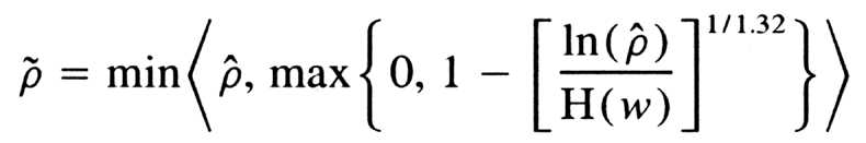
and

H (w) = min (10^-50, ß₁w^0.04 + ß₂w^0.06 + ß₃w^0.08)

where, for the LAD regression model,
 

ß = 147.85585 1
ß = 0266.53958 2
ß = 118.99034, 3

and for the LSD regression model,

ß = 155.60230 1
ß = 0279.97996 2
ß = 124.79452. 3

As an example for the LAD regression model, suppose n = 40, p = 6, w = 33, and  = 0.60. Then the estimated population  value is = 0.510. The corresponding estimate for the LSD regression model is  = 0.507. Note that the LAD ratio  /  = 0.600 / 0.510 =1.177 and the LSD ratio  /  =0.600 / 0.507 = 1.183 are estimates of artificial skill and correspond to entries in column C3/C1 of Tables 1, 2, 3, 4, and 5. Finally, it is emphasized that each estimated population  value  is merely a single estimator. If one is fortunate enough to have calculated values close to the population regression coefficients, then obviously, very little degrading will occur. On the other hand, the degrading may be more extreme than indicated by a single estimator. It is not possible to develop similar equations for shrinkage, since C4/C3 is a ratio of two random variables (C3 and C4) and no population values exist for prediction purposes - that is, the values of C1 that were used in the previous prediction models. However, when the population is not contaminated ( population 1) , it is apparent that the shrinkage is approximately twice the artificial skill. Because artificial skill and shrinkage are of diminished consequence with increasing sample sizes, it is important to update temporal datasets that exhaust all available information. This will serve to increase the sample size and, consequently, decrease both artificial skill and shrinkage.
 
 

c. Application to recent studies

The results of this study regarding the degrading of forecast skill, as measured by agreement coefficients, permit clarification and explication of previously reported forecasts. For these purposes, three studies by the authors are used to illustrate the degrading of forecast skill. Specifically, Gray et al. ( 1992, 1993, 1994) report LAD and LSD regression model nondegraded measures of agreement between various indices of tropical cyclone activity in the Atlantic basin ( including the Atlantic Ocean, Caribbean Sea, and Gulf of Mexico) : number of named storms (NS) , number of named storm days (NSD) , number of hurricanes (H), number of hurricane days (HD) , number of intense hurricanes ( IH) , number of intense hurricane days (IHD) , hurricane destruction potential (HDP) , and net tropical cyclone activity (NTC) . The values for IH, IHD, HDP, and NTC have been adjusted to reflect a small overestimation of major hurricane intensities as reported by Landsea (1993) and are identified as IH*, IHD*, HDP*, and NTC* ( cf. Gray et al. 1994) . These eight indexes of tropical cyclone activity were forecast using both LAD and LSD regression models at three points in time: 1 December, 1 June, and 1 August. The 1 December prediction was based on six predictors ( including the intercept ) and 41 years of data (Gray et al. 1992) ; the 1 June prediction was based on 14 predictors and 42 years of data (Gray et al. 1994) ; and the 1 August prediction was based on 10 predictors and 41 years of data. The 48 nondegraded measures of agreement based on the LAD and LSD prediction models at 1 December, 1 June, and 1 August for the eight indexes of tropical cyclone activity are from Gray et al. (1992, 1993, 1994) and are summarized in Table 6. Also included in Table 6 are the corresponding 48 degraded measures of agreement.

While it is clearly not possible to apply the degrading formula to a single sample, Table 6 summarizes the C3/ C1 degrading (not C4/C3 shrinkage) as applied to the original data of Gray et al. (1992, 1993, 1994) and shows what might vaguely be anticipated, on average, if the Gray et al. (1992, 1993, 1994) studies were repeated many times. Applying the degrading equation to a single sample is analogous to making a statement as to the likely truth of an individual statistical hypothesis. For example, if a type I error is set at α = 0.05, a 95% confidence interval is always a statement about the interval not about the population parameter. That is, of all intervals constructed, 95% will contain the true population parameter. However, nothing can be said about a particular interval calculated from a single sample. Any confidence that a researcher has in a particular interval is undefined probabilistically. The same is true of hypothesis testing; no inference can be made about
a particular sample. Rejection of a null hypothesis tells us nothing about the particular sample in question. However, in the long run and on average, we can expect to reject the null hypothesis when it is true about 5 in 100 times when α = 0.05.

7. The problem of validation

Because artificial skill, such as indexed in the C3/C1 column of Tables 1b, 2b, 3b, 4b, and 5b, is pervasive in most prediction research, investigators often attempt to validate their sample regression coefficients. The usual method is called                "cross-validation" in which a few observations (up to one-half the observations) are omitted, at random, from a model and the
model is then tested on the omitted observations (Michaelsen 1987) . More typically, a sample of size n is divided into a construction sample of size n -1 and a validation sample of size 1, and the model is then tested in all possible (n) ways (Stone 1974, 112) . In meteorological forecasting research, this cross-validation procedure is usually realized by withholding each year in turn and deriving a forecast model from the remaining n -1 years, checking each of the n forecast models on the year held in reserve (Livezey et al. 1990; Barnston and Van den Dool 1993; Elsner and Schmertmann 1994) . Ideally, of course, the construction model based on sample regression coefficients should be validated against several independent validation samples drawn from the population of interest, but few researchers have the luxury of a simulation study in which the entire population is known and available. Column C4 in Tables 1a, 2a, 3a, 4a, and 5a and the C4/C1 column in Tables 1b, 2b, 3b, 4b, and 5b contain the results of just such a validation study in which, it will be recalled, sample regression coefficients are applied to five new independent samples of size n, and  agreement values between the y and  values are computed for each of the five samples. With 10 000 construction samples and 5 validation samples, each entry in column C4 is the average of 50 000  values. It is abundantly clear from even a cursory inspection of the C4/C1 column in Tables 1b, 2b, 3b, 4b, and 5b that when contamination is present the LSD regression model produces inflated estimates of validation fit and expected skill.

Inspection of column C1 in Table 1a reveals that both the LAD and LSD regression models yield about the same amount of agreement between the y and  values in (the noncontaminated) population 1. Although the LAD regression model yields systematically higher agreement coefficients in every instance, the differences are slight. On the other hand, inspection of
column C1 in Table 3a reveals that the LAD and LSD regression models yield quite different amounts of agreement between the y and  values in population 3, which contains 1% severe contamination. While the LAD regression model yields slightly lower agreement coefficients when compared to the agreement coefficients in the noncontaminated population 1, the LSD regression model yields greatly reduced agreement coefficients, relative to those obtained in population 1. Because the contaminated data points in population 2 - 5 were added at the extremes of the independent variables, but cluster around the median of the dependent variable, the added data points exert a considerable amount of both leverage and influence that are magnified by the intrinsic squaring function inherent in the LSD regression model. These additional data points
have the general effect of moving the regression plane from its position in the noncontaminated population and increasing the overall sum of squared prediction errors, resulting in a lower coefficient of agreement. The LAD regression model, based on absolute deviations, is less affected by these extreme values, as reflected in its higher agreement values.

When a sample is drawn with replacement from a contaminated population, the chances are that the sample will not contain any of these extreme values, especially when the sampling fraction n/N is small. Thus, considering column C4 of Table 3a where samplebased regression coefficients are validated against five new, independent random samples, it is clear that, in most cases, successive samples are more representative of each other than they are of the population from which they were drawn. This results in higher average sample agreement values than exist in the population for the LSD regression model. The C4/C1 ratios are given in column C4/C1 of Table 3b, where it can be observed that nearly every LSD validation fit exceeds 1.0. The LAD regression model, based on absolute deviations about the median, is relatively unaffected by even 1% severe contamination, but the LSD regression model, based on squared deviations about the mean, systematically overestimates the validation fit and yields greatly inflated indexes (column C4/C1) of expected skill.

Acknowledgments.
This analysis was supported by NOAA and NSD Climate Research Grants. We appreciate the encouragement and support of Dr. David Rodenhuis and Dr. Jay Fein.
 

REFERENCES

Badescu, V., 1993: Use of Willmotts index of agreement to the validation of meteorological models. Meteor. Mag., 122, 282-286.

Barnston, A. G., and H. M. Van den Dool, 1993: A degeneracy in cross-validated skill in regression-based forecasts. J. Climate, 6, 963-977.

Copas, J. B., 1983: Regression, prediction and shrinkage. J. Roy. Statist. Soc., B45, 311-354.

Cotton, W. R., G. Thompson, and P. W. Mielke, 1994: Real-time mesoscale prediction on workstations. Bull. Amer. Meteor. Soc.,75, 349-362.

DeMaria, M., and J. Kaplan, 1994: A statistical hurricane intensity prediction scheme (SHIPS) for the Atlantic basin. Wea. Forecasting,9, 209-220.

Elsner, J. B., and C. P. Schmertmann, 1993: Improving extendedrange seasonal predictions of intense Atlantic hurricane activity. Wea. Forecasting, 8, 345-351.

, and , 1994: Assessing forecast skill through cross-validation. Wea. Forecasting, 9, 619-624.

Gray, W. M., C. W. Landsea, P. W. Mielke, and K. J. Berry, 1992:Predicting Atlantic seasonal hurricane activity 6-11 months in advance. Wea. Forecasting, 7, 440-455.

, , , and , 1993: Predicting Atlantic basin seasonal tropical cyclone activity by 1 August. Wea. Forecasting, 8, 74-86.

, , , and , 1994: Predicting Atlantic basin seasonal tropical cyclone activity by 1 June. Wea. Forecasting, 9, 103-115.

Hess, J. C., and J. B. Elsner, 1994: Extended-range hindcasts of tropical-origin Atlantic hurricane activity. Geophys. Res. Lett., 21, 365-368.

Holland, G. J., 1993: Tropical cyclone motion. Global Guide to Tropical Cyclone Forecasting, WMO/TC 560, Rep. TCP-31, World Meteorological Organization, Geneva, Switzerland, 363 pp.

Jarvinen, B. R., C. J. Neumann, and M. A. S. Davis, 1984: A tropical cyclone data tape for the North Atlantic basin, 1886-1983: Contents, limitations, and uses. NOAA Tech. Memo. NWS NHC 22, 21 pp.

Landsea, C. W., 1993: A climatology of intense (or major) Atlantic hurricanes. Mon. Wea. Rev., 121, 1703-1713.

Livezey, R. E., A. G. Barnston, and B. K. Neumeister, 1990: Mixed analog/persistence prediction of seasonal mean temperatures for the USA. Int. J. Climatol., 10, 329-340.

McCabe, G. J., and D. R. Legates, 1992: General-circulation model simulations of winter and summer sea-level pressures over North America. Int. J. Climatol., 12, 815-827.

Michaelsen, J., 1987: Cross-validation in statistical climate forecast models. J. Climate Appl. Meteor., 26, 1589-1600.

Reynolds, R. W., 1988: A real-time global sea surface temperature analysis. J. Climate, 1, 75-86.

Shapiro, L. J., 1984: Sampling errors in statistical models of tropical cyclone motion: A comparison of predictor screening and EOF techniques. Mon. Wea. Rev., 112, 1378-1388.

Stone, M., 1974: Cross-validatory choice and assessment of statistical predictions. J. Roy. Statist. Soc., B36, 111-147.

Tucker, D. F., P. W. Mielke, and E. R. Reiter, 1989: The verification of numerical models with multivariate randomized block permutation procedures. Meteor. Atmos. Phys., 40, 181-188.

Watterson, I. G., 1996: Nondimensional measures of climate model performance. Int. J. Climatol., in press.

Willmott, C. J., 1982: Some comments on the evaluation of model performance. Bull. Amer. Meteor. Soc., 63, 1309-1313.

, S. G. Ackleson, R. E. Davis, J. J. Feddema, K. M. Klink, D. R. Legates, J. Donnell, and C. M. Rowe, 1985: Statistics for the evaluation and comparison of models. J. Geophys. Res.,
90, 8995-9005.