ABSTRACT

  A surprisingly strong long-range predictive signal exists for Atlantic-basin seasonal tropical cyclone activity. This predictive skill is related to two measures of West African rainfall in the prior year and to the phase of the stratospheric quasi-biennial oscillation of zonal winds at 30 mb and 50 mb, extrapolated ten months into the future. These predictors, both of which are available by 1 December, can be utilized to make skillful forecasts of Atlantic tropical cyclone activity in the following June-November season. Using jackknife methods to provide independent testing of datasets, it is found that these parameters can be used to forecast nearly half of the season-to-season variability for seven indices of Atlantic seasonal tropical cyclone activity as early as late November of the previous year.

1. Introduction

  The Atlantic basin (including the Atlantic Ocean, Caribbean Sea, and Gulf of Mexico) experiences a larger variability of seasonal hurricane activity than does any other global hurricane basin (Gray 1985). Table 1 summarizes statistics on the year-to-year variability of various Atlantic seasonal tropical cyclone parameters. The number of hurricanes per season in recent years has ranged from 12 (1969), 11 (1950), and 9 (1955, 1980) to 2 (1982) and 3 (1957, 1962, 1972, 1983, 1987). This interannual variability suggests that large-scale climate factors acting on seasonal and longer-term time scales are involved and that some degree of seasonal predictability may be possible. Until recently, however, there has been no reliable objective method for predicting whether a forthcoming hurricane season was likely to be relatively active, inactive, or near normal.

  Recent research (Gray 1984a,b, 1990b) indicates that there are seasonal hurricane predictive signals for the Atlantic basin from global and regional predictors that are available by 1 June (the beginning of the "official" hurricane season) and by 1 August (the beginning of the most active portion of the season). Similar highly skillful predictive relationships are generally not operative or are much weaker in other tropical cyclone basins (Chan 1991; Nicholls 1984) or in the middle latitudes (Livezey 1990). The five predictors utilized for these seasonal hurricane forecasts include two slowly varying global-scale climate factors: 1) the phase of the stratospheric quasi-biennial oscillation (QBO), and 2) the presence or absence of a moderate-to-strong El Nifio event, and three persistent regional-scale factors: 3) 200-mb zonal wind; 4) sea level pressure anomalies in the Caribbean basin; and 5) the anticipated June-September rainfall in the western Sahel region of Africa. The importance of western Sahel rainfall to concurrent Atlantic-basin hurricane activity has only recently been recognized (Gray 1990a; Landsea 1991; Landsea and Gray 1992; Landsea et al. 1992). Incorporating this rainfall factor into seasonal tropical cyclone forecasts adds an additional degree of complexity in that it becomes necessary to correctly forecast western Sahel rainfall. However, the strength of the rainfall association demands that an estimate of the western Sahel rainfall be made.

  Whereas the five predictors identified above are operative at the beginning of the Atlantic hurricane season, the purpose of this paper is to analyze the two extended-range predictors of Atlantic seasonal activity that are available 6-11 months in advance. These two extended-range predictors are 1) the forward-extrapolated (10 months) strength of stratospheric QBO zonal wind near 100N latitude for September and 2) rainfall in West Africa that occurs prior to 1 December in the previous year. Currently, these are the only predictors for Atlantic tropical cyclones that have been identified to operate on such a long time scale.

  This paper separately discusses each of the stratospheric QBO and West Affican-rainfall extended-range predictors and then performs jackknife statistical analyses to determine the degree of independent 6-11 month forecast skill that is available from these two predictors.

2. QBO winds as a long-range predictor of hurricane activity

a. QBO variability

  The easterly and westerly modes of stratospheric QBO zonal winds that circle the globe over the equatorial regions have a substantial influence on Atlantic tropical cyclone activity (Gray 1984a; Shapiro 1989). About twice as much intense-hurricane activity (V_max > 50 m s^-1) occurs during seasons when the stratospheric QBO winds at 50 mb (20-km level) are in the westerly anomaly mode. As illustrated in Figs. 1 and 2, the absolute values of the zonal vertical wind shear between 50 mb (20 km) and 30 mb, (23 km) is relatively small in west-phase seasons. Table 2 shows the associations of forward-extrapolated (from November to September) stratospheric QBO zonal winds and Atlantic hurricane activity, particularly intense-hurricane activity. Note the large differences in the numbers of intense hurricane activity that occur between these two QBO stratified 15-yr groupings. Figure 3 shows the large differences in intense-hurricane tracks that are associated with these contrasting extrapolated QBO zonalwind variations.

  The physical cause of these QBO-linked differences may be due to the contrasting stratospheric horizontal wind ventilation processes across the top of the hurricane, as illustrated in Fig. 2 and discussed by Gray (1988). During the east phase of the QBO, the absolute value of the stratospheric QBO winds at latitudes of 10°-15°N are strongly from the east. This condition causes net advection of hurricane structural elements that extend into the lower stratosphere away from the hurricane center. This relative advection is likely to act to restrain the stratospheric contribution to hurricane development and intensification. By contrast, during the west phase of the QBO, the absolute value of the zonal wind in the stratosphere (over hurricanes) at 10°- 15° N is weak. In this case, comparatively small horizontal wind ventilation may occur in the lower stratosphere (Fig. 2). This west-phase condition is a positive influence on the inner-core intensity of developing hurricanes. In this way the QBO west phase is a positive cyclone influence, and the east phase a negative influence. Additionally, it is possible that the QBO exerts other dynamical influences upon the largescale environment within which the hurricanes form. These involve hydrostatic height and temperature field differences associated with east and west phases of the QBO. Recent work (e.g., Gray et al. 1992a,b) shows support for these ideas; however, continued research into the QBO-tropical cyclone association is needed.

b. Methodology for forward extrapolation of QBO

  The stratosphere QBO is special in that it may be the only atmospheric phenomena that can be extrapolated accurately ten months into the future. Although the QBO cycle is the most predictable of all long-term wind variations, it is still observed to have a 20%-30% variability in both period and amplitude. This variability inevitably leads to inaccuracies in 10-month forward extrapolations of the cycle. Two sources of error are possible in estimating the future trends in the QBO. For the purposes at hand, these include: 1 ) the proper location of the November QBO wind in relation to the current QBO wrind cycle and 2) the possible departure of the (future) tenmonth QBO trend from the changes expected based on the long-term climatology of 17 QBO cycles since 1950. These potential errors are recognized, and may not be too restrictive. We find that typically, skillful estimates of the future magnitude of the QBO zonal wind can be made ten months in advance.

  Figure 4 shows the climatology of the Balboa, Canal Zone, (9°N) stratospheric QBO zonal-wind variability (relative to the annual cycle) that occurs at 50 mb (-20-krn altitude) and at 30 mb (-23 km). These curves were constructed by averaging the periods and magnitude of each QBO relative wind shift at Balboa for the 38 years of 1950-1987. This figure can be used to specify the location (phase) of the current (i.e., November) QBO wind in relation to the full cycle. Date positioning within the QBO cycle can usually be well estimated in relation to the date of the last zero crossing (i.e., west-to-east or east-to-west phase transition). Westerly and easterly periods at 30 mb typically last about 14.5 and 13.5 months, respectively, with a bias to longer westerly and shorter easterly periods at 50 mb.

  The position of the November 30-mb and 50-mb zonal wind in relation to the phase of the QBO cycle is estimated by noting the number of months since the last reversal of sip. If, in November, 30-mb winds had switched from easterly to westerly anomalies nine months previously, then we would judge from climatology that the next westerly-to-easterly transition would occur six months later (by the next June). We would expect that by the following September the QBO would be three months into a new easterly phase of the QBO cycle. Figure 5 shows how this extrapolation would be made. Table 3 lists the duration in months of the westerly and easterly phases of the QBO at 50 mb and 30 mb prior to each November between 1950 and 1990.

  Separate extrapolations are made for the 30-mb and 50-mb levels. Once these 10-month (or current November to next September) extrapolations of the QBO winds are made, corrections for the annual wind cycle at 10°N latitude are made for each level, and estimated values for the absolute zonal winds are obtained. We find that this simple quantitative extrapolation gives accurate and reproducible estimates of September QBO winds for the following year. This ten-month extrapolation is quite easy to apply, requiring only the number of months since the previous QBO phase transition, west to east, or vice versa. The expected climatologically specified ten-month extrapolated winds for the following September can then be read from Table 4.

  The November QBO wind can also be used as an aid to adjust for longer-than-average QBO periods. For instance, the 30-mb QBO westerly wind mode is sometimes observed to persist for periods as long as 18 months. If November zonal winds are still westerly after 16 or 17 months or are still strongly westerly after 14 or 15 months, then this westerly cycle can be judged to be longer than normal. In this case, a 2-3-month backward time correction is appropriate for the November positioning within the westerly cycle. Note in Table 4 that provision is made to account for such extended period occurrences.

  Values of 10-month climatologically extrapolated 30-mb and 50-mb September zonal winds for the period of 1950-1990 are given in Table 5; values for observed winds are shown in the second column. The actual winds minus the extrapolated winds, or the extrapolation error, are given in the last column. The mean of the error for these extrapolated winds is only about 40% as large as the mean error for the September wind estimates based only on the September climatological wind. Hence, we can definitely make improved estimates relative to mean conditions using this 10-month extrapolation procedure.

3. African rainfall as a long-range predictor of hurricane activity

a. Western Sahel rainfall

  The Sahel is the transition zone between the Sahara Desert to the north and the rainforest region of the Guinea Coast. During the last few decades much of the Sahel has experienced large year-to-year persistent rainfall anomalies (Nicholson 1979). In general, wet years were followed by wet years (e.g., in the 1950s and 1960s), while dry years often follow dry years (e.g., in the 1970s and 1980s). This persistence provides a moderate amount of skill for the forecasting of Atlantic hurricane activity because of the strong concurrent association of western Sahel rain to Atlantic basin hurricanes (Gray 1990a; Landsea 1991; Landsea and Gray 1992; Landsea et al. 1992).

  Utilizing data from 38 western Sahel rainfall stations (Fig. 6) that are described in Undsea and Gray (1992), a standardized index of western Sahel rainfall has been constructed during the two wettest months of August and September. This index is made of the average of the standardized deviation of each station. Note how most of the years of the 1950s and 1960s were wet, while those of the 1970s and 1980s were dry. Yearly values of this index are shown in Fig. 7 and listed in Table 1.

  Figure 7 shows the strong multidecadal rainfall variations that have affected the western Sahel since the late 1960s. Such multidecadal controls on West African rainfall are likely linked to long-term (interdecadal) sea surface temperature anomaly patterns around the globe (Folland et al. 1986). It is also possible that the persistence of low rainfall (especially during the
drought-stricken 1970s and 1980s) has contributed to natural changes of the land surface (Nicholson 1988) and to related anthropogenic alterations in the land surface, such as overgrazing and deforestation (Chamey 1975). Either of these effects may contribute to alterations of the West Aftican monsoonal circulation, and, hence, of the embedded squall lines, as a result of differences in surface moisture availability and land-surface temperature.

  Table 6 gives statistical information on the hurricane activity during seasons one year after each of the ten wettest and each of the ten driest western Sahel August and September periods between 1949 and 1989. Note the modulation of the hurricane activity wherein there is only a modest difference in the total number of hurricanes, but a nearly two to one (wet/dry) difference for the seasonal incidence of intense hurricane days. Figure 8 portrays differences in the intense- (category 3-4-5) hurricane tracks for these two ten-year rainfall classes. Note the many more intense-hurricane tracks in the Atlantic in the area to the east of Florida during wet rather than dry years.

b. Gulf of Guinea rainfall

  Landsea (1991) has documented a surprisingly strong predictive signal for seasonal intense Atlantic hurricane activity based on August-November rainfall along the Gulf of Guinea of the previous year. As with the Sahel rainfall data, rainfall from 24 Gulf of Guinea locations (shown in Fig. 6) is combined in terms of the mean standardized deviation for the region. Figure 9 presents the yearly variations in this rainfall index for 1949-1990.

  The variations in seasonal hurricane activity 6-11 months after each of the ten wettest and each of the ten driest August-November periods in the Gulf of Guinea rainfall are shown in Table 7. This extendedrange association appears to be the strongest of any of the individual predictors. Note that in the ten hurricane seasons following the ten wettest Gulf of Guinea periods, the rate of intense-hurricane days activity was four times the level of that which occurred during the hurricane seasons following the ten driest Gulf of Guinea periods, and the number of intense hurricanes was 2.6 times as many. This difference is also reflected in Fig. 10. where the composited tracks of individual intense hurricanes are shown for both the ten wettest and the ten driest Gulf of Guinea seasonal periods. Landsea (1991) has shown that the strong correlations between these rainfall data and the seasonal hurricane data are unaffected by a linear detrending of both datasets.

  The strong association realized between the Atlantic basin hurricane activity and prior-year Gulf of Guinea rainfall is likely due to feedbacks on the monsoon circulation from one year to the next. As discussed by Landsea (1991), heavy rainfall along the Gulf of Guinea as the summer monsoon retreats southward from August to November may provide an enhanced moisture source that contributes to a strong onset of the next vear's monsoon. This moisture may be available through soil moisture and evapotranspiration from the biosphere. Thus. abundant rainfall along the Gulf of Guinea may lead to more rain in the Sahel during the follo,,ving year and greater Atlantic basin hurricane activitv. Conversely, a drier August to November period along the Gulf of Guinea may contribute to drought in the Sahel several months later. Such droughts are typically associated with much reduced intense-hurricane activity (Fig. 10).

In the following section we perform independent statistical tests on stratospheric QBO and West African rainfall data for the 41-yr period from 1949 through 1989 to determine the extent (skill level) to which the QBO and West African rainfall data can be used for long-range (ten-month lead time) seasonal hurricane forecasts.

4. Analyses and results

  The statistical methodology for the analysis of the data consists of four distinct, but interrelated, steps:

  1 ) Least-absolute deviation regression provides prediction values, based on a forecast model, for each of the n = 41 yr.
In the construction of any forecast model, it is imperative that the model be aeveloped on a subset of the data and then independently tested on a different subset of the data that was not used In the formulation of the model. This cross validation of a forecast model may be accomplished by means of a jackknife procedure.

  2) A cross-validation (jackknife) procedure ensures that the prediction for any year is independent of the
observations for that year. Since the purpose of the present methodology is to forecast a single year, n - 1 = 41 - 1 = 40 yr of data are used for the formulation of each forecast model, and each model is then tested on the remaining 1 yr of independent data not used in the construction of the model. This procedure is repeated 41 times, yielding 41 prediction values for each of 7 seasonal dependent variables.

  3) The cross-validated prediction values and the observed values for each of the n = 41 yr are compared by calculating a measure of agreement.

  4) The probability of the measure of agreement is obtained under the null hypothesis. Details of this statistical methodology are presented in appendix B.

  The prediction equation for each of the seasonal dependent variables (i.e., named storms, named storm davs. hurricanes, hurricane days, intense hurricanes, intense-hurricane days, and hurricane destruction potential ) is
 
 

where  represents one of the seven dependent variables, 0 ,1 , and 2 are the LAD regression weights determined from a nonjackknife solution (see appendix B), W is a composite function of the extrapolated (November to September) upper-air zonal winds at 50 mb (U₅₀) and 30 mb (U₃₀), where

and R is a composite function of August-September western Sahel (R_s) and August-November Gulf of Guinea (R_G) rainfall, where

The weights (a₁, a₂, a₃, a₄, and a₅) for each of the predictor variables are given in Table 8 for each of the dependent variables. These weights were empirically determined, with LAD regression and the jackknife solution, to maximize the agreement coefficient () described in appendix B.

  The agreement coefficients () and their associated probability values (P) are given in Table 9. For comparative purposes only. the corresponding values of the squared Pearson cross-product correlation coefficient ( r² ) are presented in the last column of Table 9. Since the results of Table 9 are based on the cross-validated LAD criterion, the values of r² are not maximized. While r² is strictly a measure of linearity (i.e.. r² = 1 implies all observed and predicted value pairs fall on a line that does not necessarily have a unit slope or pass through the origin),  is a measure of agreement. and  = 1 implies all observed and predicted value pairs fall on a line with unit slope that passes through the origin. Thus, the values of r² are often larger than the corresponding values of ; since r² depends on squared Euclidean distance residual values. r² can be smaller than  (Mielke 1984). The fact remains that r² is not a satisfactory measure of agreement. (Incidentally, had the jackknifed predictors been replaced with the nonjackknifed predictors, then all values of  and r² in Table 9 would have been larger. These larger values of  and r² are inappropriate, however. since independent validations of the predictions are necessary.)

  In order to predict future results, regression weights (0 ,1 , and 2) are required. Using 1 ) the jackknife solution weights for the predictor variables (a₁, a₂, a₃, a₄, and a₅), 2 ) LAD regression, and 3 ) a nonjackknife solution, the regression weights were calculated. Table 10 gives the regression coefficients for each dependent variable for future predictions. (Because the values of  and  r² given in Table 9 are based on crossvalidated LAD predictors, they will be smaller than the corresponding values of  and r² based on the nonjackknife regression coefficients in Table 10.)
Substituting (2) and (3) into ( 1 ) yields the prediction equation given by

As an example of the seasonal forecasts, the coefficients of Tables 8 and 10 yield the following prediction equation for the seasonal number of intense hurricanes (IH):

  The diagrams of Fig. 11 present the scatter plots of the predicted values of each of the seven predictors versus the observed values. While the dependence between predicted and observed values is visually apparent, this empirical model is obviously imperfect. When a prediction is negative, as observed for HD, IH, IHD, and HDP, a zero should, of course, replace a predicted negative value. A further feature specifically involving IH, IHD, and HDP is that the models tend to underestimate observed values that are extremely large. Awareness of this underestimation bias and the negative forecasts allows one to subjectively alter the cases in question, and a somewhat higher forecast skill may be obtained.

  Note in Table 9 that we can independently (jackknife) hindcast over 44% of the measure of agreement value () for all seven forecast parameters. In fact, we can hindcast over 49% of the value of  for the seasonal number of named storm days, number of intense hurricanes, and number of intense-hurricane days. The probability that there is no hindcast statistical skill in any of these forecast parameters is between 10^-5 and 10^-8.

5. Discussion

  It is remarkable that Atlantic s easonal hurricane activity, manifesting itself as sporadic mesoscale events, would show such a strong association with forcing functions so far removed in space and time. This association is further evidence for the primary role of global and regional circulation patterns in governing seasonal hurricane frequency and intensity. Recent research by Gray (1988) and others further illustrates the fundamental role of the large-scale and global circulation patterns in determining the frequency and the intensity with which the smaller-scale mesoscale weather events are able to develop into hurricanes. Previously, we had viewed hurricanes, along with the weaker weather systems that spawned them, as the product of rapidly varying local circulation characteristics that had a large random component and that were impossible to predict a few days in advance, let alone ten months in advance. Although this view is still true for individual hurricane systems, it does not hold for the seasonal aggregate of hurricane systems. The climate signal has a strong influence in determining the number of short-lived and transitory events (i.e., hurricanes) that may be activated.

  It was not expected that such strong relationships between climate and hurricanes would exist and have such longperiod lag responses. If, in the future, the atmosphere continues to behave as it has over the last 41 yr, then a considerable amount of extended-range future seasonal forecast skill is available. We have no reason for thinking that the atmosphere will not continue to behave during the next few decades as it has during the last four decades. Forecast skill during the first 20-yr period differed little from the last 21 -yr period.

  Skillful extended-range prediction, at least of Atlantic seasonal hurricane activity, is indeed possible. Considering the difficulties inherent in any seasonal weather-prediction scheme plus the extraordinary 611 -month extended range of this relationship, we consider this to be an important finding. Until recently, few serious researchers would have imagined that there might be seasonal predictive signals this strong extending this far into the future. In addition, full exploitation of all potential Atlantic predictive signals has not yet been made. Further study of additional unexploited regional or global variables, including West African land temperatures, land and ocean surface pressure, Atlantic SSTs, plus other potential seasonal predictors, have not yet been accomplished. Consequently, it is most likely that further improvements are possible with additional research.

  Acknowledgments. The authors wish to thank Richard Taft and William Thorson for their very expert assistance in the processing of the West African rainfall data and to John D. Sheaffer for many beneficial discussions and for assistance in manuscript preparation.

  We are very grateful for the West African rainfall data supplied to us by William Spangler andRoy Jenne of the National Center for Atmospheric Research (NCAR). Much of the data came from the extensive African rainfall collections originally compiled by Sharon Nicholson of Florida State University, Graham Farmer of the US AID/Fews Project, Peter Lamb of the University of Oklahoma, Douglas Le Comte of the US AID program, Dave Miskus and R. J. Tinker of the NOAA Climate Analysis Center, and E. 0. Oladipo of Ahmodu Bello University of Nigeria. James Angell provided QBO wind information. Barbara Brumit and Laneigh Walters provided expert assistance in manuscript preparation and data analysis.

  This research was supported primarily by a climate grant from the National Science Foundation, with
supplemented assistance from the NOAA Office of Global Programs.

Atlantic basin. The area including the entire Atlantic Ocean, the Caribbean Sea, and the Gulf of Mexico.

Tropical cyclone (TC). A large-scale circular flow occurring within the tropics and subtropics that has its strongest winds at low levels, including hurricanes, tropical storms, and other weaker rotating vortices.

Tropical storm. A tropical cyclonewith maximum sustained winds between 39 (18 ms^-1 or 34 kt) and 73 (32 ms^-1 or 63 kt) miles per hour.

Named storm (NS). A hurricane or a tropical storm. Named storm day (NSD). Four 6-h periods during which a tropical cyclone is observed or estimated to have attained tropical-storm or hurricane-intensity winds.

Hurricane (H). A tropical cyclone with sustained lowlevel winds of 74 miles per hour (33 ms^-1or 64 kt) or greater.

Hurricane day (HD). Four 6-h periods during which a tropical cyclone is observed or estimated to have hurricaneintensity winds.

Intense hurricane (IH). A hurricane reaching at some point in its lifetime a sustained low-level wind of at least 111 mph (96 kt or 50 ms^-1). This constitutes a category 3 or higher on the Saffir-Simpson scale (Simpson 1974).

Intense-hurricane day (IHD). Four 6-h periods during which a hurricane has intensity of Saffir-Simpson category 3 or higher.

Hurricane destruction potential (HDP). A measure of a hurricane's potential for wind and storm-surge destruction defined as the sum of the square of a hurricane's maximum wind speed for each 6-h period of its existence.
Values are given in 0.25 X 10⁴ (ms^-1)².

Saffir-Simpson (S-S) category. A measurement scale ( 1-5 ) of a hurricane's wind and ocean-surge intensity. One is the weakest hurricane, 5 the most intense hurricane (Simpson 1974).

APPENDIX B

Statistical Methodology

  The statistical methodology for the analysis of the data consists of four distinct, but interrelated, steps: 1 ) Leastabsolute deviation regression provides prediction values for each of the n years. 2) A cross-validation (jackknife) procedure ensures that the prediction for any year is independent of the observations for that year. 3) The crossvalidated predicted values and observed values for all n years are compared by calculating a measure of agreement. 4) The probability that the observed measure of agreement occurred by chance alone (the null hypothesis) is obtained.

  Ordinary least-squares (OLS) regression analysis yields efficient and unbiased estimates of population regression parameters and their associated standard errors when the population is Gaussian (or multivariate Gaussian) with equal variances (or a variance-covariance matrix that exhibits compound symmetry). The OLS is far from optimal in many non-Gaussian situations, especially when the population distribution is asymmetric and/or when outlying values are present. Even a modest departure from a Gaussian distribution can seriously degrade the efficiency of OLS estimates (Kowalski 1972; Rey 1983; Micceri 1989). The problems generated by non-Gaussian distributions and/or extreme values are common in weather and forecast data. One of the most satisfying robust alternatives to OLS regression is least-absolute deviation (LAD) regression (Barrodale and Roberts 1973, 1974-, Bloomfield and Steiger 1980; Dielman 1984; Gentle et al. 1977; Mielke 1987; Narula and Wellington 1982-, Seneta 1983). The LAD regression, which predates OLS regression (Sheynin 1973), is analogous to the use of the median in a univariate analysis to estimate the location of a distribution, since the median minimizes the sum of the absolute values of the residuals. For this reason, LAD regression estimates are 1 ) far more efficient than OLS estimates whenever the median is a better estimator of location than the mean and are 2) exceedingly more resistant than OLS regression to extreme values. As documented elsewhere (Mielke 199 1; Sheynin 1973), C. F. Gauss (circa 1809) was unable to obtain the numerical solutions needed for LAD regression, and had to develop OLS regression as a default procedure. (Even though Gauss developed linear programming to implement LAD regression, the lack of any computational support made him realize that a simple calculus solution could implement OLS regression.)

  To evaluate the prediction values of LAD regression, a cross-validation procedure is required. For any given year, the LAD prediction values are calculated from all remaining years when the dependent and independent observations of the given year are removed. This procedure is repeated for each of the n distinct years in question, and ultimately provides n independently predicted values.

  The n observed values and the n corresponding predicted values are compared to see if they agree (i.e., are identical). The measure of agreement utilized in the analysis is a chance-corrected measure based on absolute differences between the n pairs of observed and predicted values (Berry and Mielke 1988; Mielke 1984,1991).

  Finally, the statistical significance of the agreement measure is determined. The observed measure of agreement value is compared against all possible values of the measure by obtaining the probability of having a value as large or larger than the observed measure of agreement under the null hypothesis.

 For simplicity, let y_i, denote the dependent variable and let x_i1, . . . , x_ir, denote r independent variables associated with the ith of n events. Let _i, denote the predicted value of y_i based on the r independent variables. In addition, _i is termed the cross-validated predictor of y_i since _i is determined only from the n - 1 remaining events when the ith event is removed. Each _i, is calculated from its associated LAD regression, where

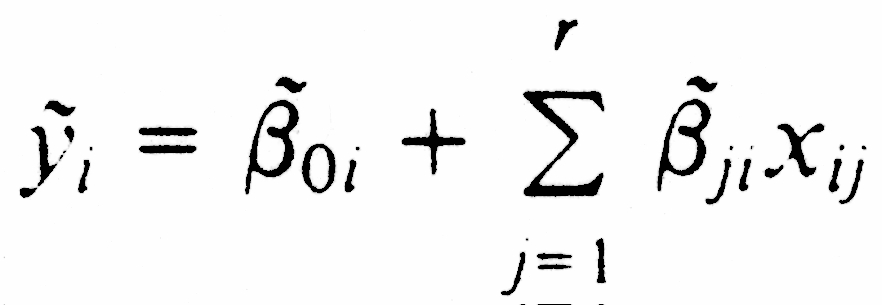
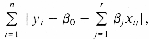
for i =1, . . . . , n and ( _0i,_li, . . . _ri) are those values of ( _o, ₁, . . . _r) that minimize the sum of n - 1
absolute differences given by

denotes the sum of all events except the ith event). Furthermore, the nonjackknifed predictor of y for future events is given by

where ( _o, ₁, . . . _r) are those values of ₀,₁, . . . . , _r that minimize the sum of n absolute difference givein by
 
 

that is the, nonjackknifed predictor of y () depends on all n events. The choice of LAD regression instead of OLS regression is that LAD regression is geometricallv consistent with the data in question (Mielke 1985, 1986, 1987, 1991 ).The linear programming algorithm used to obtain the LAD regression estimates is due to Barrodale and Roberts ( 1973, 1974). The permutation procedure used to evaluate each regression is based on the statistic given by

Thus, is the dispersion between yi and i (the jackknifed predictor of i ) averaged over the n events. The observed value of  (denoted by ₀) is compared with the n! possible values of  where all n! orderings of 1, . . . n are associated with the observed sequence 1, . . . ,n. The null hypothesis dictates that all n! possible values of  are equally likely. Under the null hypothesis, the significance of o is given by

The accuracy of the n jackknifed predicted values (1, . . . .n), where each jackknifed prediction depends on
the n - 1 independent events using the previously described cross-validation procedure, requires a comparison with the n corresponding observed values (y₁, . . . y_n). A measure of agreement between the corresponding y₁ and _i, values based on  is given by

where ^u is the expected value of  under the null hypothesis. If  = 1, then perfect agreement is achieved (note that  = 0 implies that y_i  = _i, for i = 1, . . . , n), whereas p < 0 implies no agreement. The process is continued until the cross-validation procedure's LAD estimates maximize the measure of agreement. Algorithms, computer programs, and discussion involving the P value and  are given elsewhere (Berry and Mielke 1988; Iyer et al. 1983; Mielke 1984, 199 1; Mielke and Iyer 1982). A closely related alternative criterion to maximizing  is minimizing . The difference between these two criteria is that maximizing  is a nonlinear criterion ( depends on the regression coefficients). whereas minimizing  is a linear criterion.
 
 
 

REFERENCES

Barrodale. I. and F. D. K. Roberts. 1973: An improved algorithm for discrete L₁ linear approximation. S.I.A..11. J. Numer. Anal.. 10, 839-848.

-, and -, 1974: Solution of an overdetermined system of equations in the L, norm. Commun. Assoc. Comp. Mach- 17, 319-320.

Berry. K. J.. and P. W. Mielke. 1988: A generalization of Cohen's kappa agreement measure to interval measure and multiple raters. Educ. Psych. Meas., 48, 921-933.

Bloomfield, P., and W. Steiger, 1980: Least absolute deviations curve fitting. Sci. Statist. Comput..1, 290-301.

Chan, J. C. L., 199 1: Prediction of seasonal tropical cyclone activity over the western North pacific. Preprints, Fifth Conf on Climate Variaiions, Denver, Amer. Meteor. Soc., 521-524.

Charney, J. G., 1975: Dynamics of desert and drought in the Sahel. Quart, J. RoY. ffeteor. Soc., 101, 193-202.

Dielman, T. E., 1984: Least absolute value estimation in regression models: An annotated bibliography. Commun. Stat., A13, 513-541.

Folland, C. K., T. N. Palmer, and D. E. Parker, 1986: Sahel rainfall and worldwide sea temperatures, 1901-85. Nature, 320, 602607.

Gentle, J. E., W. J. Kennedy, and V. A. Sposito, 1977: On least absolute deviations estimations. Commun Statist., A6, 839845.

Gray, W. M., 1984a: Atlantic seasonal hurricane frequency. Part 1: El Nifici and 30 mb quasi-biennial oscillation influences. Afon. Wea. Rev., 112, 1649-1668.

-, 1984b: Atlantic seasonal hurricane frequency. Part 11: Forecasting its variability. Mon. Wea. Rev.. 112, 1669-1683.

-1985: Tropical yclone global climatology. WMO Tech. Document WMO/TD-No. 72, Vol. 1, WMO, Geneva, Switzerland, 3-0.

-, 1988: Environmental influences on tropical cyclones. Aust. Afeteor. 11ag., 33, 127-139.

-, 1990a: Strong association between west African rainfall and U.S. landfalling intense hurricanes. Science, 249, 1251-1256.

-, 1990b: Summary of 1990 Atlantic tropical -cyclone activity and seasonal forecast verification. Colorado State University, Department of Atmospheric Science. Fort Collins, CO, 29 pp.

-, J. D. Sheaffer, and J. A. Knaff, 1992a: A mechanism for the modulation of ENSO variability by the stratospheric QBO. J. Meteor. Soc. Japan,

-, - and -, 1992b: Hypothesized mechanism for stratospheric QBO influence on ENSO variability. Geophys. Res. Lett., 19, 107-110.

Iyer, H. K., K. J. Berry, and P. W. Mielke, 1983: Computation of finite population parameters and approximate probability values for multiresponse randomized block permutation procedures (MRBP). Commun. Slat., B12,479-499.

Kowalski, C. J., 1972: On the effects of non-normality on the distribution of the sample product-moment coffelation coefficient. Appl. Stat., 21, 1-12.

Landsea, C. W., 1991: West African monsoonal rainfall and intense hurricane associations. Department of Atmospheric Science. Paper No. 484, Colorado State University, Ft. Collins, CO, 272 PP.

, and W. M. Gray, 1992: The strong association between westem Sahel monsoon rainfall and intense Atlantic hurricanes.
J Climate, 5, 435-453.

, C.W., W.M. Gray, P.W. Mielke, Jr., and K.J. Berry, 1992: Long-term variations of Western Sahelian monsoon rainfall and intense U.S. landfalling hurricanes. J. Climate, 5, 1528-1534.

Livezey, R. E., 1990: Variability of skill of long-range forecasts and implications for their use and value. Bull. Amer. Meteor. Soc., 71,300-309.

Micceri, T., 1989: The unicom, the normal curve, and other improbable creatures. Psych. Bull., 105, 156-166.

Mielke, P. W., 1984: Meteorological applications of permutation techniques based on distance functions. Handbook of Statistics, Vol. 4: Nonparametric Methods, P. R. Krishnaiah and P. K. Sen. Eds., North-Holland Publishing Co., 813-830.

, 1985: Geometric concerns pertaining to statistical tests in the atmospheric sciences. J Atmos. Sci., 42, 1209-1212.

-, 1986: Non-metric statistical analyses: Some metric altematives. J. Stat. Plann. Inference, 13, 377-387.

-, 1987: L1, L2 and L. regression models: Is there a difference? J. Stat. Plann. Inference, 16, 430.

- 1991: The application of multivariate permutation methods based on distance functions in the earth sciences. Earth-Sci. Rev., 31,55-71.

- and H. K. Iyer, 1982: Permutation techniques for analyzing multi-response data from randomized block experiments. Commun. Stat., All, 1427-1437.

Narula, S. C., and J. F. Wellington, 1982: The minimum sum of absolute errors regression: A state of the art survey. Int. Stat. Rev., 50, 317-326.

Nicholls, N., 1984: Predictability of interannual variations of Australian seasonal tropical cyclone activity. Mon. Wea. Rev., 113, 1144-1149.

Nicholson, S. E., 1979: Revised rainfall series for the West African subtropics. Mon. Wea. Rev., 107, 620-623.

-, 1988: Land surface-atmosphere interaction: Physicad processes and surface changes and their impact. Progr. P~vs. Geogr., 12, 36-65.

Rey, W. J. J., 1983: Introduction to Robust and Quasi-Robust Statistical Methods. Springer-Verlag.

Seneta, E., 1983: The weighted median and multiple regression. Aust. J. Stai., 25, 370-377.

Shapiro, L. J., 1989: The relationship of the quasi-biennial oscillation to Atlantic tropical storm activity. Mon. Wea. Rev., 117, 1545-1552.

Sheynin, 0. B., 1973: R. J. Boscovich's work on probability. Arch. Hist. Exact Sci., 9, 306-324.

Simpson, R. H., 1974: The hurricane disaster potential scale. Weatherwise,_27, 169-186.